
MOBILE SENSORGROUP WITH SMART PATH FOR
DETECTING TARGET AREA
Kuen-Liang Sue and Jing-Wei Lin
Department of Information Management, National Central University, Taoyuan, Taiwan
Keywords: Mobile Sensor Networks, Incremental Clustering, Exploration.
Abstract: The aim of this study is to design an intelligent mechanism for exploring unknown target areas in a plant,
such as oil pollution in ocean. To explore the target area efficiently, a smart sensing mechanism based on
Incremental Clustering algorithm is proposed to cooperate with a small sensing network structure named
Centralized SensorGroup (CSG). The operation processes and detection phases are provided and verified in
the investigation. System performance is evaluated by observing the detection completeness and accuracy in
different scenarios within a square experimental area of 100m*100m. No matter when large or small
scenarios are explored, simulation results demonstrate that CSG cooperated with the smart sensing
mechanism has quite good detection accuracy and efficiency and can achieve the purpose of exploring
target area efficiently and effectively.
1 INTRODUCTION
With the development of robot and wireless
transmission technologies, mobile sensors (MS) can
provide mobility for wireless sensor networks and
mobile sensor networks can be formed through
various wireless interfaces
(Liang et al, 2006; Dantu
et al, 2005
; Hu and Evans, 2004). Mobility of
mobile sensor networks brings some significances
and potentials. Mobility can let the sensor network
moves to collect information in the environments
that traditional fixed sensor networks can not be
deployed (Clark, 2005; Casbee et al, 2006; Wang et
al, 2005). One of the application issues of mobile
sensor network is to detect and localize specific
target areas in the sensing environment, for example,
the detection of oil spoiled area in the ocean
environment. Traditional sensor networks detect
environment by random deployment. However, due
to the higher cost of MS, it is inappropriate to use
mobile sensor network by the same way. Hence,
how to use few MS nodes to detect unknown target
areas efficiently is a key issue in this application.
The aim of this study is to design an intelligent
mechanism for exploring unknown target areas in a
plant, such as oil pollution in ocean. To detect the
targets efficiently, a smart sensing mechanism based
on Incremental Clustering algorithm is proposed to
cooperate with a small sensing network structure
named Centralized SensorGroup (CSG).
The remainder of this paper is structured as
follows. Because we use incremental clustering
algorithm to improve the efficiency of detection, the
related data clustering techniques is introduced
briefly in section 2. The proposed mobile sensor
network structure and sensing mechanism are
described in section 3. Simulation method and
numerical analyses are described in section 4.
Section 5 provides conclusion for the investigation.
2 BACKGROUNDS
In this study, we propose a sensing mechanism
designed for a small mobile sensor network to detect
the unknown target areas in the environment. The
proposed mechanism utilizes a skill for data mining
called cluster analysis to offer sensor network the
ability to analyze the distribution of target area from
sensing records and adjust the movement of CSG
dynamically by using data clustering algorithms.
Hence, the exploration job can be performed more
efficiently and effectively.
Cluster analysis is an unsupervised machine
learning technology. Clustering algorithms’
operation is based on the concept of grouping the
similar data into a cluster and making the data in
different clusters dissimilar (Jain et al, 1999). The
36
Sue K. and Lin J. (2010).
MOBILE SENSORGROUP WITH SMART PATH FOR DETECTING TARGET AREA.
In Proceedings of the International Conference on Wireless Information Networks and Systems, pages 36-41
DOI: 10.5220/0002981100360041
Copyright
c
SciTePress
traditional techniques are mainly designed for static
databases environment. For example, the K-means
algorithm is one of the traditional partitioning
clustering algorithms (Law and Jain, 2005). The
general objective is to obtain a fixed number of
clusters and minimizes the total square errors of the
all clusters.
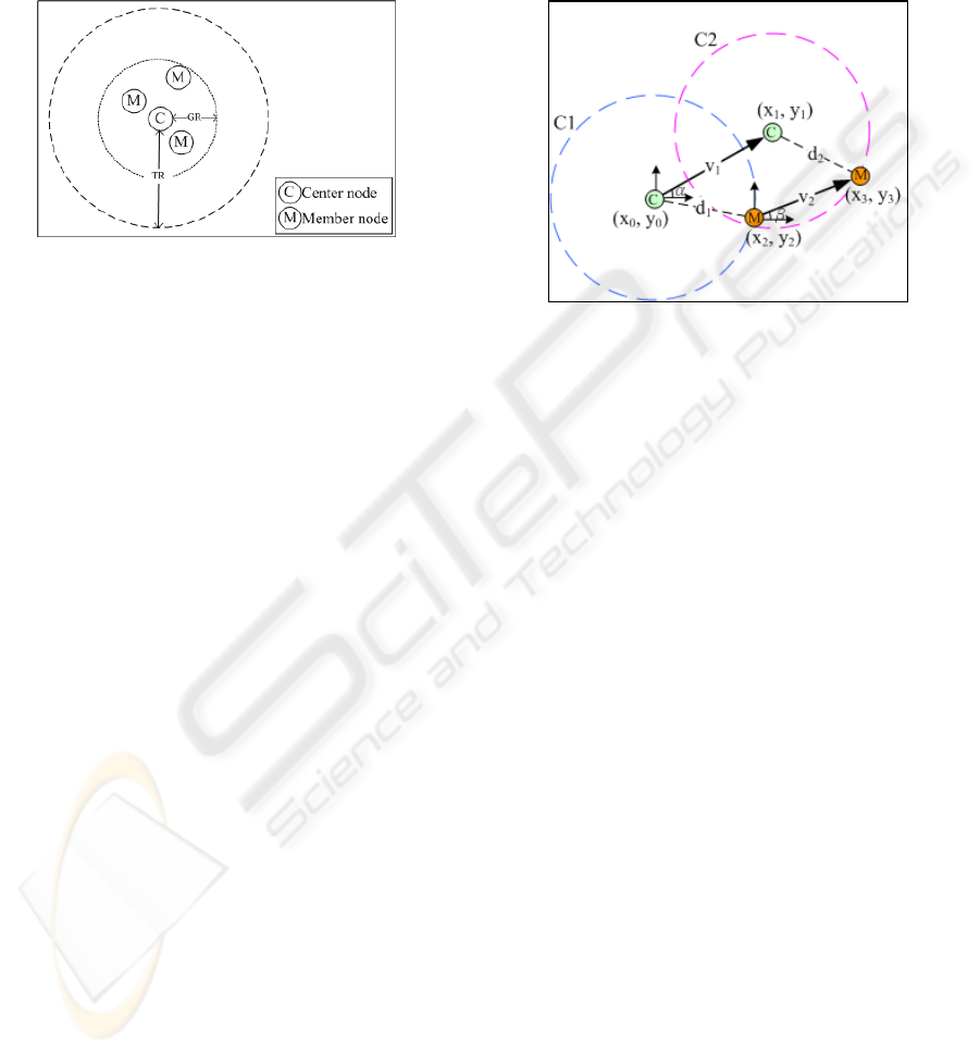
Figure 1: CSG structure.
However, with the increasing requirements of
data clustering, the limits of traditional data
clustering algorithms exist due to that they usually
need to load all data into memory while analyzing.
To solve the problem, incremental clustering
algorithms are proposed for the dynamic database
environments (Ester et al, 1998; Pons-Porrata et al,
2005). Incremental clustering algorithms executes
clustering analysis whenever a data enters the
database, thus these algorithms can cluster all data
by executing simple calculations instead of loading
all data into memory and executing complicate
analysis. That is, incremental clustering algorithm
needs fewer requirements for computation resource
and ability. The proposed exploration mechanism is
supposed to cooperate with mobile sensors which
are usually assumed to have limited computing
resources. Therefore, incremental clustering
algorithm is appropriate to be used for activating the
sensing mechanism in the proposed sensing
networks.
3 EXPLORATION SCHEME
To detect the targets efficiently, the mobile sensors
should be formatted to a network and operate as a
group basing on a systematic sensing mechanism.
Thus this study is composed with two parts - mobile
sensor network structure and sensing mechanism.
3.1 Centralized SensorGroup
Centralized SensorGroup (CSG) is a mobile sensor
network structure constructed with number of MS
nodes crowded within a specific range. The concept
of CSG is to let CSG keeps moving in the
environment. MS nodes in a CSG keep detecting
targets while moving. If a MS detects the border of
target, then it records its current location as a
sensing record. Finally, the location of targets’
borders can be known by using the sensing records.
Figure 2: Initial phase.
In the following parts, we introduce the CSG
structure and CSG’s operation process.
3.1.1 CSG Network Structure
The movement of MS in CSG is based on Reference
Point Group Mobility (RPGM) (Hong et al, 1999).
According to the functions of MS in CSG, there are
two roles of MS in CSG called Center node (C node)
and Member node (M node). As shown in Fig. 1, C
node is the MS allocated in the center of CSG. It is
responsible of controlling all operations of CSG and
broadcasting its location to all M nodes within its
transmission range (TR) periodically. M nodes are
the other MS deployed surround C node. They move
randomly surround C node within the range of group
range (GR). In CSG structure, only C node requires
GPS ability. C node acts as a mobile anchor in the
network and other M nodes can calculate their
locations by using a wireless localization algorithm.
We assume that all MS in CSG should be equipped
with a compass to measure the direction of its
movement and have the ability to measure the
distance of its movement.
3.1.2 Localization Algorithm of CSG
The localization algorithm used in CSG is modified
from the algorithm proposed (Akcan et al, 2006). In
this algorithm, all mobile nodes within a group
exchange their information with each other and
calculate their local coordinates in the group basing
MOBILE SENSORGROUP WITH SMART PATH FOR DETECTING TARGET AREA
37
on the information to keep their group moving. In
this study, we modify this algorithm and combine it
with CSG structure. There are two phases
in the modified algorithm, the “initial phase” and the
“verification phase”.
In the initial phase, C node broadcasts its
location with packets Loc1 and Loc2 at time t1 and
t2 sequentially. As shown in Fig. 2, C node adds its
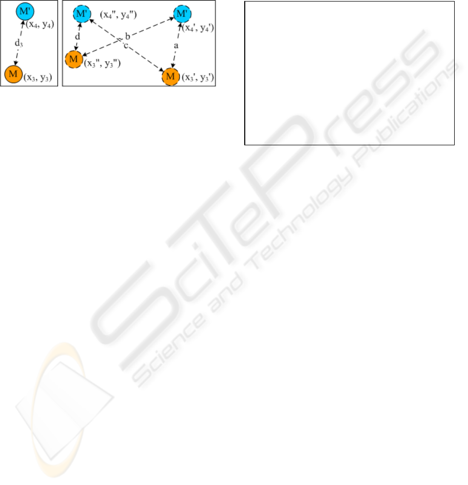
Figure 3: Verification phase.
location (x0, y0) into Loc1 and broadcasts it to all M
nodes at time t1. An M node can measure the
distance to C node d1 by TOA (Time Of Arrival)
when it receives Loc1. After t1, C node and M nodes
start moving along the directions they decided. At
time t2, C node then broadcast its location (x1, y1)
with Loc2 again and an M node measures the
distance to C node d2 when it receive Loc2. After
the above process is finished, an M node can
calculate two circles C1 and C2 by using the
coordinates (x0, y0), (x1, y1) and the distance d1,
d2. These two circles define the sets of possible
locations of an M node at t1 and t2. Because M node
can calculates it displacement vector from t1 to t2, it
can calculates a new circle C1’ by displacing C1
with the vector (v2cosβ, v2sinβ). Because both C1’
and C2 define the set of possible locations of M
node at t2, M node can get its t2 candidate locations
by calculating the intersection of C1’ and C2.
In the verification phase, each M node exchanges
its t2 candidate locations with each other by
broadcasting a VeriInfo packet. When an M node
receives VeriInfo from other one, it firstly measures
the distance to the sender, then verifies an answer
from its candidate locations by using this distance.
Finally, M node calculates a weight for the verified
answer. For example, as shown in Fig. 3 (a), M
receives a VeriInfo packet from M’. M firstly
measures the actual distance d3, and then uses d3 to
verify the most possible candidate. As shown in Fig.
3 (b), M can compose at most four sets of candidate
location by using the t2 candidate locations of M and
M’. Then M compares the distances of four
candidate sets a, b, c and d with d3 and chooses the
set which has smallest difference with d3 as the
verified answer. Then M gives this answer a weight
value by calculating the inverse of the difference of
the chosen candidate set distance and the actual
distance d3. As shown in Fig. 3 (b), the candidate set
with the distance value “a” has the smallest
difference with d3, so M chooses (x3', y3') as the
verified answer of the VeriInfo packet from M’ and
gives (x3', y3') a weight by calculating 1/|d3– a|. An
Figure 4: CSG operation procedure.
M node can choose one of its candidates and gives
the one a weight value whenever it receives a
VeriInfo. The weight value for each candidate
location is accumulated. Finally, M can get the t2
localization result by calculating the weighted mean
of its candidate locations and can also get t1
localization result by using its displacement vector
from t1 to t2 in the initial phase.
3.1.3 CSG Operation Process
The CSG operation procedure and communi-cation
protocol between CSG members are shown in Fig. 4.
In the initial of operation, CSG is firstly set to the
initial location (step 1). Then C node starts moving
with speed Vc and leads CSG to detect targets (step
2). CSG iterates step 4-14 with a period of T seconds,
this periodical process is called a “RPGM round”. In
this process, C firstly gets its GPS location Lc and
broadcast Lc with a RPGMbroadcast packet to all M
nodes (step 4-5). When an M node receives a
RPGMbroadcast (step 7), it firstly executes the
process to end the n-1th RPGM round. This process
includes the localization result determination of n-
1th RPGM round (step 8) and the conversion of the
temporary sensing records in n-1th RPGM round
(step 9). In step 9, due to that M nodes in CSG can’t
get their current locations timely, all sensing record
in n-1th RPGM round are temporarily stored as the
displacement vectors from time t
1
to the time they
detect the border of target. After the t1localization
(
b
)
(
a
)
Centralized SensorGroup procedure
1. Set initial location of CSG
2. C moves with speed V
c
3. iterate every T seconds period
4. L
c
Å GPS location of C
5. C RPGMbroadcast ( L
c
)
6. for each M do
7. Receives L
c
form C
8. Location determination
9. Records conversion
10. L
m_init
Å initial location
11. L
m_dest
ÅRandom destination
12. M moves with speed V
m
13. CSG Localization process
WINSYS 2010 - International Conference on Wireless Information Networks and Systems
38
result is determined in step 8, M nodes convert the
temporary sensing records in n-1th RPGM round to
actual sensing record by adding t
1
localization result
to all temporary records. M node then starts the
process of nth RPGM round. It calculates the initial
location L
m
_
init
of nth RPGM round by adding t
2
localization result of n-1th RPGM round with the
displacement form t
2
to the time it receive
RPGMbroadcast of nth RPGM round (step 10).
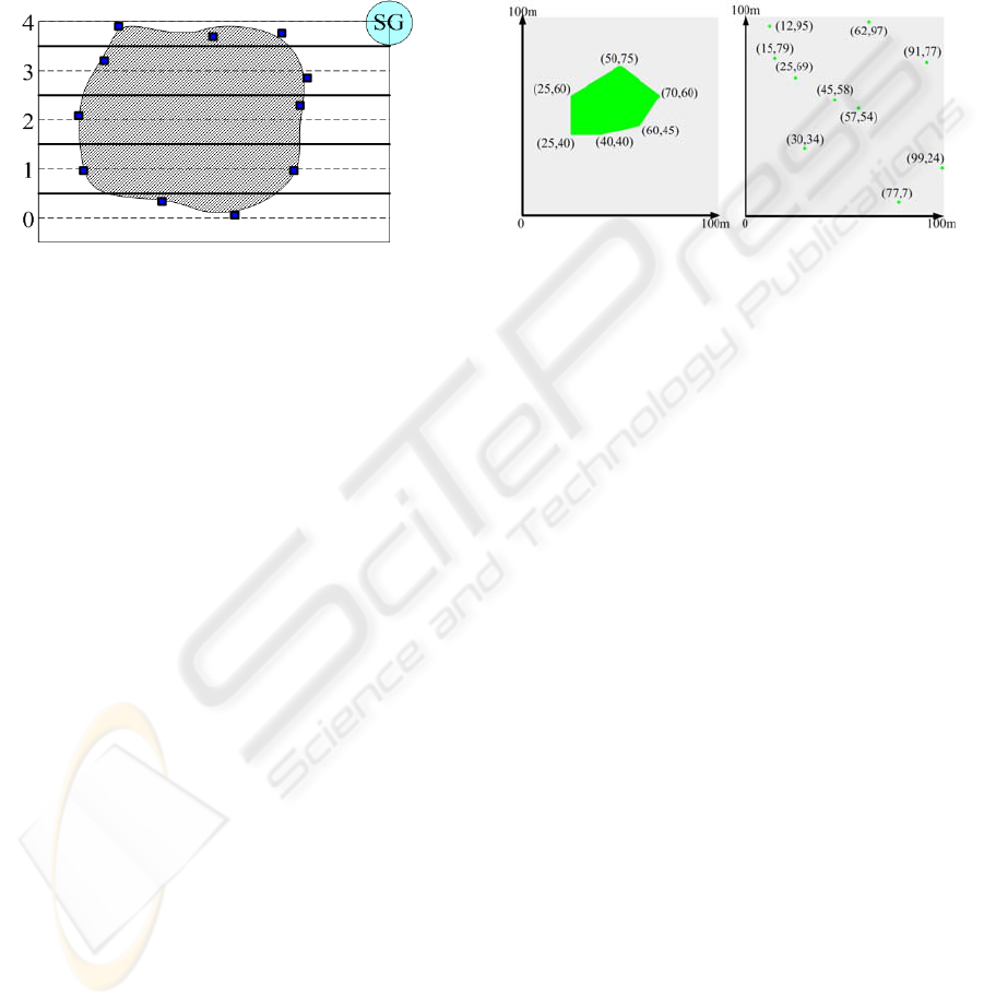
Figure 5: Concept of data collection phase.
Then M node decides a random destination L
m
_
dest
around L
c
within range of GR (step 11) and starts its
movement with speed V
m
(step 12). CSG then
executes the localization process of nth RPGM
round (step 13), C node sends Loc1 after
RPGMbroadcast immediately at t
1
. After T seconds,
C node broadcasts RPGMbroadcast again to end the
nth and start the n+1th RPGM round.
3.2 Sensing Mechanism
To detect the unknown targets in the environment, C
node need a systematic sensing mechanism to
control the moving path of CSG. An Incremental
Clustering Aided Sensing Mechanism (ICASM) is
proposed in this study. In this mechanism, we
assume that there is no obstacle in the environment.
There are two phases in a round of ICASM’s
operation. The first phase is “data collection phase”.
CSG executes a quick scan of the whole
environment to analyze the rough locations of the
targets’ borders. The second phase is “Detailed
detection phase”. CSG make a detailed detection
along the rough location of targets’ borders
according to the analysis of the first phase.
In the data collection phase, C node splits the
whole square sensing environment into number of
rectangle regions with the width of GR*2. The
centerlines of the regions are the C node’s moving
paths in this phase. C node leads CSG to scan the
environment along these paths. Because it is
possible that CSG can’t detect the borders of each
region effectively, C node splits the regions with an
interlaced style in odd and even round of ICASM.
According to the split regions, the border of
unknown target can also be split into number of
deformed lines. We expect that all sensing records
collected in this phase should be clustered basing on
these lines, each lines can own one or more clusters.
Finally, as shown in Fig. 5, C node can catch the
rough location of the target’s border by using the
(a) Single large area (b) Discrete small area
Figure 6: Scenario setting.
centroid of each cluster. To reduce the load of C
node to cluster records, a simple incremental
clustering algorithm is used as the clustering method
in this mechanism.
4 SIMULATIONS
4.1 Scenario Settings
The environment in the simulation is a 100 m*100 m
square area. There are two types of target area
deployed in the sensing environment. The first is
“single large target area”, as shown in Fig. 6 (a), the
coordinates are the apexes of target. The other is
“discrete small target area”, as shown in Fig. 6 (b),
each target is a rhombus with width and height of 2
m and the coordinates are the centroid of each target.
4.2 Parameter Settings
We use NS2 as the simulation platform. The
simulation time is 6000 seconds. A CSG network is
composed of one C node and three M nodes; the
transmission range of a node is 15 m, the period of a
RPGM round is 1 second, the speed of C node and
M nodes are 3 m/s and 5 m/s and the range of CSG
is 2 m. In the localization algorithm of CSG, the
execution time of initial phase and verification phase
in a RPGM round are 0.9 and 0.1 second.
In the localization algorithm of CSG, each MS
MOBILE SENSORGROUP WITH SMART PATH FOR DETECTING TARGET AREA
39
uses wireless signals and compass to measure the
distance between each them and their moving
directions. Both of them may be influenced by
interferences in environment. To simulate the
interferences from environment, random distance
error and angle error are added into the localization
process to analyze the effect of different level of
interferences. The range of distance error is -10% to
10% and range of angle error are -10 to 10 degrees.
Accuracy of GPS is assumed always accurate.
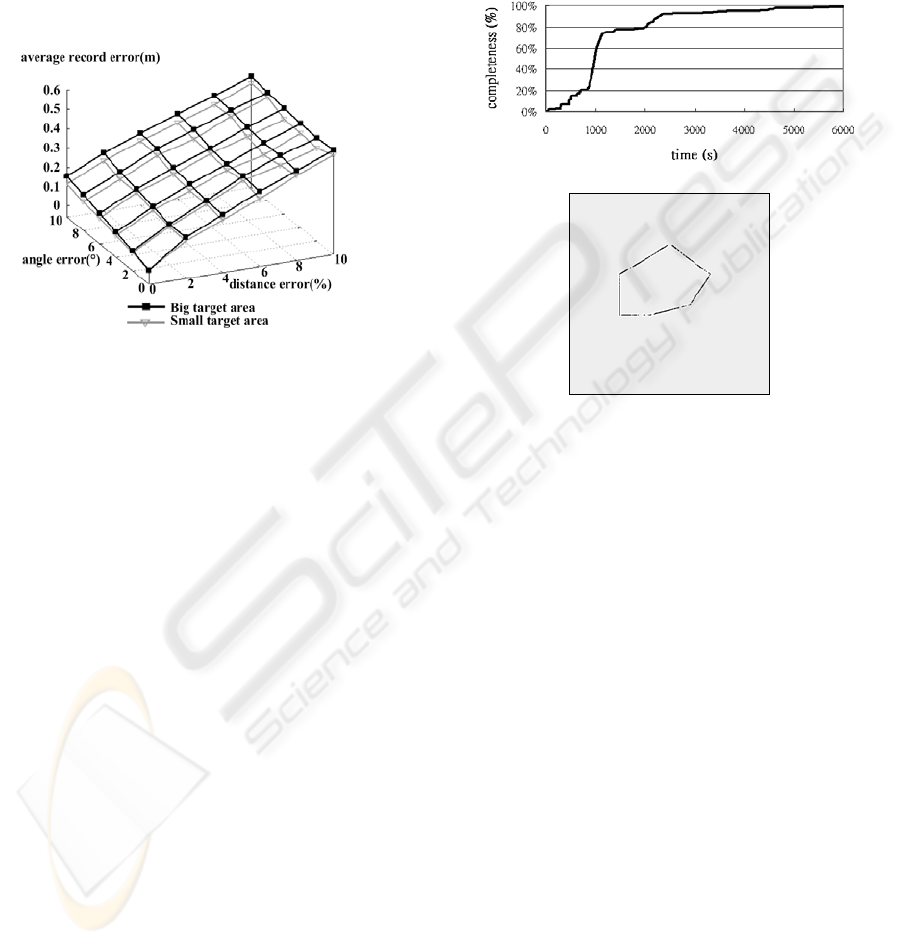
Figure 7: Detection accuracy.
4.3 Simulation Analysis Methods
We use “detection accuracy” and “detection
completeness” to analyze the detection performance
of CSG. The detection accuracy is evaluated by
calculating the average error of all sensing records
collected by CSG. We define the error of a sensing
record as the shortest distance for the record to the
border of target area.
To evaluate the of detection completeness are set
anchor coordinates on the border of target per 0.2m.
If one or more sensing record exists around an
anchor within 0.2 m, we set the status of the anchor
to “sampled”. Hence, we evaluate the detection
completeness by calculating the ratio of the number
of sampled anchor and the total number of anchor
after matching the anchor coordinates with all
sensing records.
4.4 Simulation Results
4.4.1 Detection Accuracy
Because the sensing records are mainly collected by
the M nodes, the detection accuracy is decided by
the localization accuracy of M nodes. The average
detection accuracy of CSG structures using ICASM
in two target area scenarios is shown in Fig. 7. We
can see that the increasing localization error of M
nodes in CSG lifts the error of sensing records and
decreases the detection accuracy. The average error
of sensing records in single large target scenario and
discrete small targets scenario are 0.52 m and 0.48 m
when the distance error and angle error are set to
10% and 10 degrees. In both scenarios, the higher
level of interferences is, the lower detection
accuracy in CSG becomes.
(a) Detection completeness with time
(b) Detection result for 80% completeness
Figure 8: Detection completeness in large scenario.
4.4.2 Detection Completeness
In this part, we evaluate the relationship of detection
completeness and detection time of CSG using
ICASM in both two scenarios without interferences
(0 distance error and 0 angle error). Fig. 8 (a) is the
relationship of detection completeness and detection
time in single larger target scenario. The average
time of a round in ICASM is 1195 seconds and the
average detection time required to achieve 80%
detection completeness is 2258 seconds. During the
first round, because ICASM only detects the targets
roughly in the first phase, so the trend of detection
completeness increases slowly. However, in the
second phase, ICASM can let CSG to make a
detailed detection according to the analysis of first
phase. Thus the detection performance of ICASM
increases significantly in this phase. Beside, the
trend of detection completeness in ICASM can still
increase efficiently after the first round. This means
that ICASM can adjust the movement of CSG and
achieve the purpose of efficient detection. Fig. 8 (b)
is a 80% detection completeness graphic result of
sensing records collected by CSG in once simulation.
The detection time is 2234 seconds.
WINSYS 2010 - International Conference on Wireless Information Networks and Systems
40
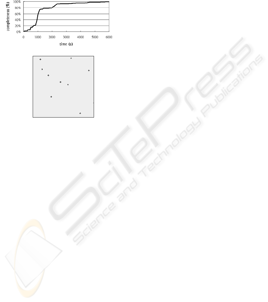
Fig. 9 (a) is the relationship of detection
completeness and detection time in discrete small
targets scenario. The average time of a round in
ICASM is 1139 seconds and the average detection
time required to achieve 90% detection
(a) Detection completeness with time
(b) Detection result for 90% completeness
Figure 9: Detection completeness in small scenariois 2353
seconds. Fig. 9 (b) is a 90% detection completeness
graphic result of sensing records collected by CSG in once
simulation. The detection time is 2215 seconds.
5 CONCLUSIONS
To identify target areas automatically is an important
application of mobile sensor networks, especially in
abnormal environment such as oil pollution in
oceans. The research investigates the problem by
utilizing small mobile sensor network. Centralized
SensorGroup (CSG) organized with several sensor
nodes, only one of them called center node needs to
be equipped with GPS functionality. During the
exploring process, GPS-free member nodes can
localize themselves by computing information from
center node and their historic data. Hence, the sensor
network is rather cost-effective. Furthermore, a
sensing mechanism based on the incremental
clustering algorithm is also proposed to adjust the
moving direction of CSG dynamically according to
the distribution of the target area. The proposed
sensing mechanism can achieve the target area
exploration more efficiently.
The detection performance is evaluated by
detection completeness and accuracy for different
scenarios in a 100m*100m square environment. The
simulation results show that. The average detection
times to achieve 80% detection completeness are
2258 seconds for large polygon scenarios. In
discrete small target scenarios, the average detection
times to achieve 90% is 2353 seconds. The average
record errors which represent the detection accuracy
in different scenarios vary between 0.48m and
0.52m. To sum up, simulation results demonstrate
that CSG cooperated the ICASM has quite good
detection accuracy and efficiency.
ACKNOWLEDGEMENTS
The research was supported by the National Science
Council, Taiwan, under the contract NSC 98-2410-
H-008-004.
REFERENCES
Liang, Y. et al. (2006). A Review of Control and
Localization for Mobile Sensor Networks.
Proceedings of Intelligent Control and Automation, 2,
9164-9168.
Dantu, K. et al. (2005). Robomote: enabling mobility in
sensor networks. Proceedings of Information
Processing in Sensor Networks, 404-409.
Hu, L. and Evans, D. (2004). Localization for mobile
sensor networks. Proceedings of the 10th conference
on Mobile computing and networking, 45-57.
Clark, J. and Fierro, R. (2005). Cooperative hybrid control
of robotic sensors for perimeter detection and tracking.
2005 American Control Conference, 5, 3500–3505.
Casbee, D. W. et al. (2006). Cooperative forest fire
surveillance using a team of small unmanned air
vehicles. International Journal of Systems Sciences,
37(6), 351-360.
Wang, G. et al. (2005). Sensor relocation in mobile sensor
networks. Proceedings of the 24th IEEE Computer
and Communications Societies, 4, 2302-2312.
Jain, A. K. et al. (1999). Data Clustering: A Review. ACM
Computing Surveys, 31(3) 122-130.
Law, H. C., Jain, A. K. 2005. Data Clustering: A User’s
Dilemma. Proceedings of Pattern Recognition and
Machine Intelligence, 3776, 1-10.
Ester, M. et al. (1998). Incremental Clustering for Mining
in a Data Warehousing Environment. Proceedings of
Very Large Databases, 24-27.
Pons-Porrata, A. et al. (2005). An Incremental Clustering
Algorithm Based on Compact Sets with Radius α.
Proceedings of Progress in Pattern Recognition,
Image Analysis and Applications, 3773, 518-527.
Hong, X. et al. (1999). A group mobility model for ad hoc
wireless networks. Proceedings of the 2nd
international workshop on Modeling, Analysis and
simulation of wireless and mobile systems, 53–60.
Akcan, H. et al. (2006). GPS-Free node localization in
mobile wireless sensor networks. Proceedings of the
5th international workshop on Data engineering for
wireless and mobile access, 35-42.
MOBILE SENSORGROUP WITH SMART PATH FOR DETECTING TARGET AREA
41
