
A COMPETING ALGORITHM FOR GRADIENT BASED
ROUTING PROTOCOL IN WIRELESS SENSOR NETWORKS
Lusheng Miao, Karim Djouani, Anish Kurien and Guillaume Noel
French South African Institute of Technology, Tshwane University of Technology
Staatsartillarie Road, Pretoria, South Africa
Keywords: Wireless sensor networks, Gradient-based routing, Energy efficiency.
Abstract: The energy consumption is a key design criterion for the routing protocol in wireless sensor networks. Some
routing protocols deliver the message by point to point like wire networks, which may not be optimal to
maximise the lifetime of the network. In this paper, a competing algorithm for GBR in wireless sensor
networks is proposed. This algorithm is referred to as GBR-C. Furthermore auto-adaptable GBR-C routing
protocol is proposed. The proposed schemes are compared with the GBR protocol. Simulation results show
that the proposed schemes give better results than GBR in terms of energy efficiency.
1 INTRODUCTION
Wireless Sensor Networks (WSNs) consist of
intelligent sensor nodes with sensing, computation,
and wireless communications capabilities. Routing
in WSNs is challenging since sensor nodes are
strongly constrained in terms of energy,
computational power, and storage capacities. The
limited energy supply is critical for the development
of WSNs. As a result, the core question to be
answered for WSNs is to determine how to save
energy in order to prolong the lifetime of the
network.
Gradient-based routing (GBR) is a routing
protocol for WSNs proposed by C. Schurgers and
M.B. Srivastava (2001). Al-Karaki, J.N and Kamal,
A.E (2004) prove that GBR is reliable in choosing
the shortest route to a sink while balancing the
energy of the whole network. However,
shortcomings exist in the GBR scheme such as
nodes which deliver the message in a point to point
manner and do not use the broadcast nature of
wireless networks. Wireless sensors are usually
equipped with omnidirectional antennas and are
placed environement with potential of data
retransmissions are high. This in turn significant
multipath transmissions so that if one node sends a
message, all its neighbors have the potential of
receiving this message. However, due to the
characteristics of the wireless channel, the number
greatly affects the energy consumption of the
network. The retransmission can be reduced if the
best node, which has already received this message,
can be selected from its neighbors to transmit this
message forward. However, very little research has
focused on GBR in term of energy saving by
considering the effect of the retransmission. Hence,
in this project, a competing algorithm which uses the
broadcasting nature of the wireless environment is
developed to improve GBR in terms of energy
efficiency.
The rest of the paper is organized as follows. In
Section 2, related work is discussed.The energy
consumption of GBR is analyzed in Section 3. In
Section 4, the competing policy and the energy
consumption analysis are proposed; furthermore an
auto-adaptable GBR-C protocol is proposed.
Simulations and results are presented in Section 5.
Conclusions and future work are given in Section 6.
2 RELATED WORK
The basic idea of competing algorithm is to exploit
the spatial diversity of the wireless medium by
involving a set of candidate forwarders instead of
only one in traditional routing, and then one
forwarder which has already received the packet is
chosen as the actual relay.
82
Miao L., Djounai K., Kurien A. and Noel G. (2010).
A COMPETING ALGORITHM FOR GRADIENT BASED ROUTING PROTOCOL IN WIRELESS SENSOR NETWORKS.
In Proceedings of the International Conference on Wireless Information Networks and Systems, pages 82-89
Copyright
c
SciTePress
H. Fussler, et al., (2003) propose a contention-
based forwarding scheme (CBF), in CBF the source
node broadcast packet to all its neighbours and then
select one best node to forward the packet.
Furthermore, the authors propose three suppression
algorithms, Basic suppression scheme, Area-based
suppression and Active selection, to prevent multiple
next hops and thereby packet duplication. However,
duplication still occurs in Basic suppression scheme
and Area-based suppression, Active selection can
prevent all forms of packet duplication but with
additional overhead.
M. Zorzi and R. R. Rao (2003) propose a novel
forwarding technique based on geographical location
of the nodes involved and random selection of the
relaying node via contention among receivers. The
receivers which are closer to the destination have the
higher priority to forward the packet, which also
means that the closer nodes to the destination are
always selected and overused.
S. Biswas and R. Morris, (2005) propose ExOR,
an integrated routing and MAC protocol that
increases the throughput of large unicast transfers in
multi-hop wireless networks. ExOR operates on
batches of packets, the source nodes includes a list
of candidate forwarders in each packet, prioritized
by closeness to the destination, the receivers with
highest priority forward packets, and then the
remaining forwarders forward the packet which
were not forwarded by the higher priority forwarders.
K. Zeng, et al., (2008) propose an algorithm to
set the forwarder priorities depending on the
expected advancement (EPA) rate in order to
achieve the maximum end-to-end throughput.
All of these works do not consider the energy
efficiency of the network, and the source node
broadcast the packet to all its neighbours which
wastes the energy of the nodes. K. Zeng, et al.,
(2007) propose an EPA per unit energy consumption
model, which calculates the best number of
forwarding candidates to broadcast the packet in
order to achieve the best energy efficiency. However
in this model, the source node needs the knowledge
of the real time delivery reliability for each
neighbour which is hard for the real wireless sensor
networks.
3 ENERGY CONSUMPTION
ANALYSIS
It is known that limited energy supply is a very
critical restriction for WSNs and that routing
protocols used in WSNs should cater for this feature.
In this section the energy consumption of GBR is
analyzed. Shortcomings in the protocol are exposed.
0
1
1
1
1
1
2
A
B
F
D
G
E
C
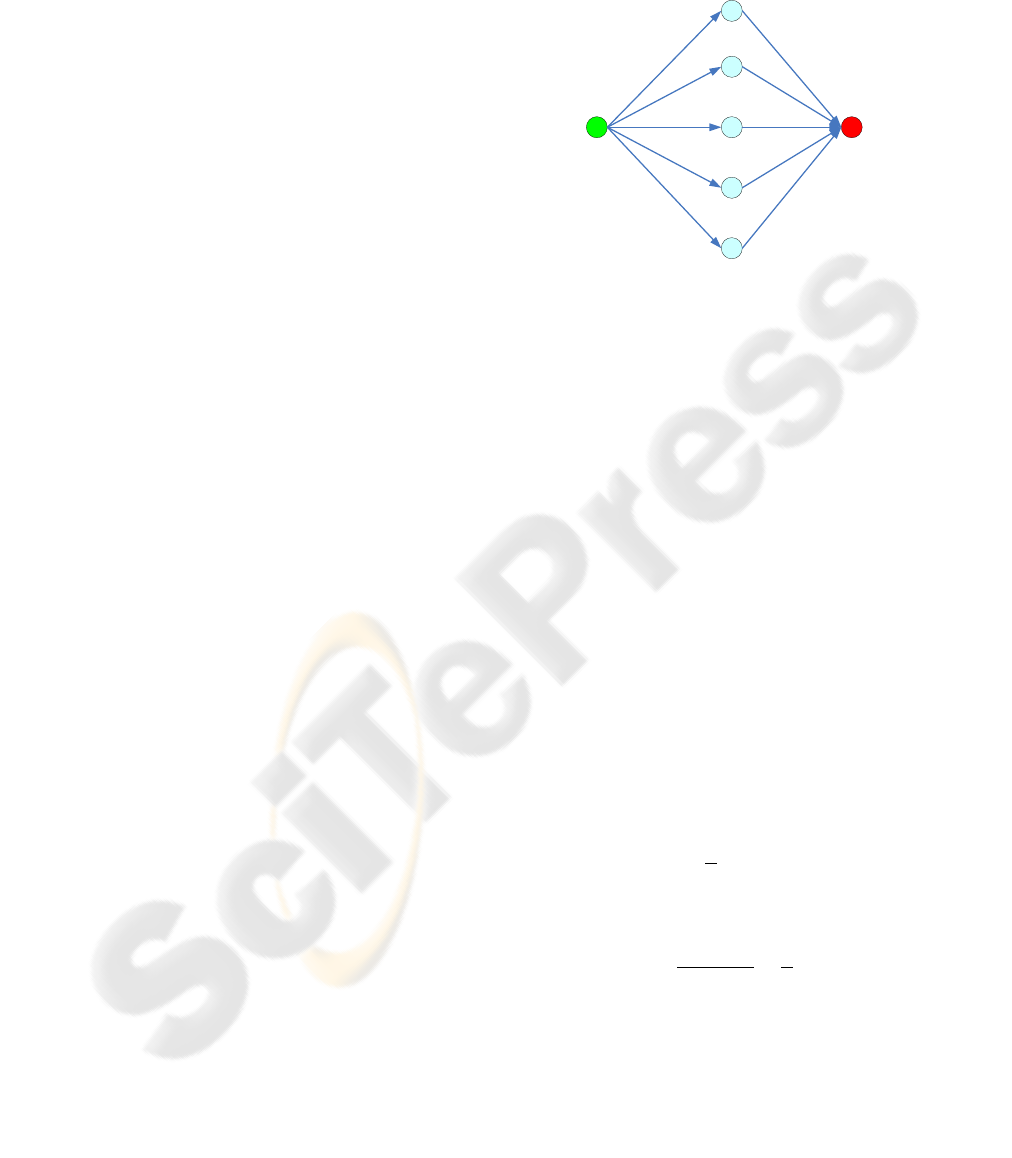
Figure 1: Two hop wireless sensor network.
Considering a simple two hop wireless sensor
network as shown in Figure 1, Node A has five next
hop nodes (determined by back propagation in GBR)
and needs to send a message to node G. In the GBR
framework, node A chooses one next hop node
among node B, C, D, E or F. Assuming the power
consumption of sending is
while the energy
overhead of receiving is
. Assume that the data
message size is M and the bit rate is Bitrate. The
transmission probability p is referred to as the
probability for one link that the receiver receives the
message successfully. To simplify the problem, the
energy consumption for the data transmission is only
considered and the other energy consumptions are
ignored. The one hop transmission energy
consumption for GBR can be determined as
. (1)
Where is the transmission time and can be
determined as
.
(2)
Equation (1) and (2) can be rewritten as
(3)
However, it can be seen that node A has five
next hop nodes. Due to the broadcast characteristic
of wireless, any of the node A’s neighbour could
receive node A’s message. As a result, if node A
sends the data to more than one next hop nodes,
assuming that the number of next hop nodes is n,
A COMPETING ALGORITHM FOR GRADIENT BASED ROUTING PROTOCOL IN WIRELESS SENSOR
NETWORKS
83
then the probability that at least one next hop node
received the data is
(4)
The one hop transmission energy consumption
can be determined from (3) and (4) as
(5)
When n=1, equation (5) is equivalent to equation
(3). Equation (5) and (3) can be rewritten as
(6)
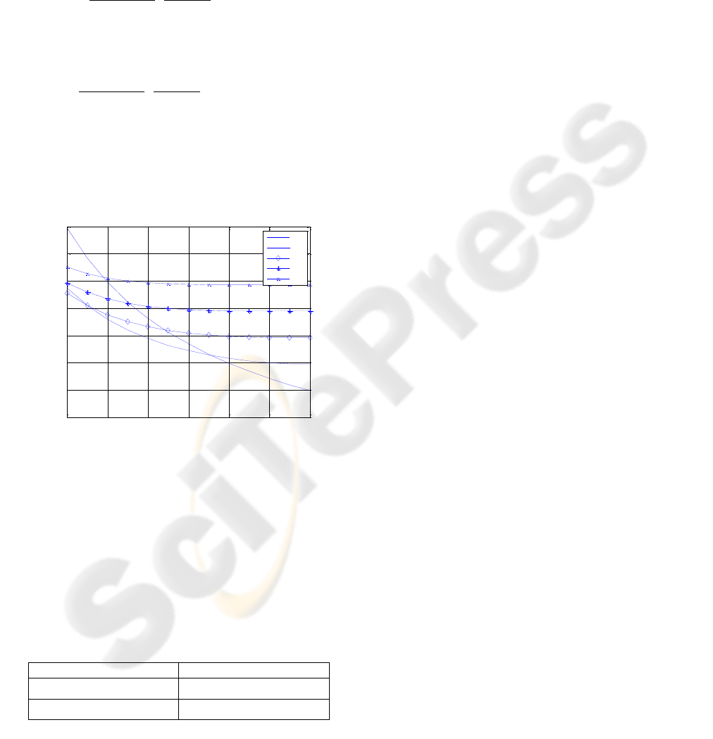
Assuming the Mica2 power consumption model
(Shnayder.V, et al., 2004) is used and p is set as
, then the energy consumption for n
from 1 to 5 can be determined. The results obtained
are shown in Figure 2.
Figure 2: The energy consumptions (
,
, M=800 bits, Bitrate=19200 bits/sec.).
It can be seen that energy can saved if we set n=2
for P<0.75. This can save up to 23% energy for one
hop transmission. Furthermore, it can be also seen
that it is enough to set at most two next hop nodes
when. In this work, the setting up of at
most two next hop nodes according to the
transmission probability P as shown in Table.1 is
considered.
Table 1: Next hop nodes number.
Transmission Probability
Next Hop Nodes Number
n=1
n=2
4 COMPETING ALGORITHM
In Section 3, it was shown that the transmission
energy can be saved by adapting the next hop nodes
number. However in real networks, we need to know
which node should transmit the data forward. For
example, in Figure 1, assume that node A needs to
send a data packet to node G. Suppose node A has
already chosen node C and D as its next hop nodes.
Then, between node C and D, it should be
determined which node should transmit the data
packet to node G. To solve this problem, a
competing algorithm for GBR is designed.
4.1 Competing Algorithm
Before the competing algorithm is discussed, the
communication model used and the three kinds of
message used are defined.
Reliable Communication Model: This implies
that the communication is such that the messages are
guaranteed to reach their destination complete and
uncorrupted. Some special measures are taken to re-
send information that did not arrive the first time.
For example, transmission is made reliable via the
use of sequence numbers and acknowledgments.
DATA: This refers to the data packet which
needs to be transmitted through the network.
ACK&DACK: These are the transmission
control characters used to indicate that a transmitted
message was received uncorrupted or without errors.
The receiver sends an ACK or DACK to the sender
depending on the destination nodes number of the
received message. If the message only has one
destination node, then the receiver sends an ACK.
Otherwise it sends a DACK.
TOGO: This is a signal that asks a node to
transmit the data message forward.
In WSNs, the messages are delivered through the
network by multi-hop and reliable communication is
very important for each hop transmission. Hence, in
this paper, wireless sensor networks which work
with reliable communication model are focused on.
The details of the competing algorithm are
shown in Figure 3:
1) The source node sends a data message to
receiver(s).
2) The receiver receives the message. If the
message is received successfully, then it
will check the destination address list of
this message.
0.4 0.5 0.6 0.7 0.8 0.9 1
3
4
5
6
7
8
9
10
P
Energy (mw)
n=1
n=2
n=3
n=4
n=5
WINSYS 2010 - International Conference on Wireless Information Networks and Systems
84
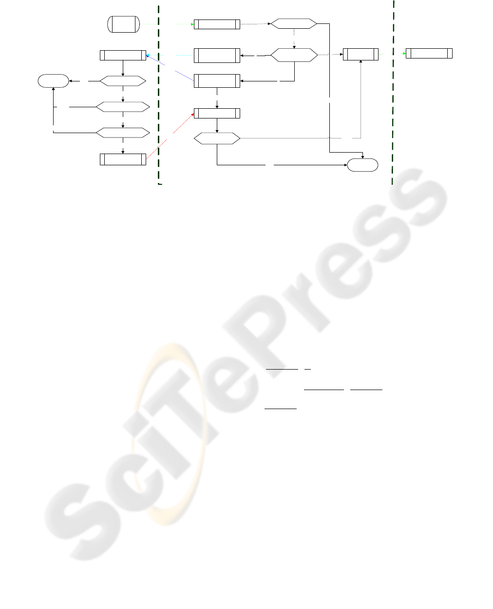
Sending
DATA
Receiving
succeed
DATA
YES
Destinatio
n number
Sending
ACK
Sending
DACK
Sending
DATA
2
Receiving
DATA
1
1
DACK
ACK
Receiving
ACK/DACK
Succeed?
YES
DELETE
NO
ACK
DACK
Is it first?
YES
NO
Sending
TOGO
TOGO
YES
Waiting T
Received
TOGO?
YES
NO
DELETE
NO
Source (Node A)
Receiver(s)
(one or two of node B C D E F)
Sink (Node G)
Figure 3: The competing algorithm flow chart.
3) If the destination address number is one,
then the receiver transmits this message to
the sink immediately. In addition, for the
reliable communication network, the
receiver also needs to send an ACK
message to the sender.
4) If the destination address number is two,
then the receiver sends a DACK message to
the source. Then a waiting time T (for
example 1s) is set.
5) The source receives the message and then
checks the message type. If it is an ACK
message, it then deletes it. If it is a DACK
message, then the source node checks if it is
the first DACK message for the data
message which it sent before. If it is the
first, then the source node sends a TOGO
message to the sender of the DACK
message. Otherwise, it deletes it.
6) If the receiver receives a TOGO message in
the waiting time T, then it transmits the
message to the sink; otherwise, deletes the
message.
The above algorithm which adopts a competing
algorithm for the GBR protocol is referred to as
GBR-C.
4.2 Energy Consumption Analysis
In section 3, the energy consumption for one hop
transmission was discussed. However, only the data
transmission was focused on. As a result, the
analysis was not very comprehensive and accurate.
In this section the energy consumption with the
competing algorithm is analyzed.
The same power consumption model used in
Section 3 is used. The ACK&DACK message size is
(D)ACK=32 bits, the Togo message size is Togo=
32 bits. In addition, compared to the data message,
the ACK and Togo message is very short. As a result,
their packet error rates are much lower than the data
message’s., In this case, we do not consider their
packet error rates.
Considering the ACK&DACK and Togo
messages, the energy consumption for GBR-C is
determined from (6) as
(7)
If we set , then the energy
consumption for GBR and GBR-C can be
determined. The results obtained are shown in
Figure 4.
It can be seen that energy can be saved if GBR-C
is used when P<0.71. A saving of up to 22% energy
for one hop transmission is seen when p=0.4. As a
result, it can be concluded that GBR-C can save
energy when the transmission probability P is less
than a certain threshold. The threshold may be
different for different application networks. For this
example, the threshold is 0.71.
A COMPETING ALGORITHM FOR GRADIENT BASED ROUTING PROTOCOL IN WIRELESS SENSOR
NETWORKS
85
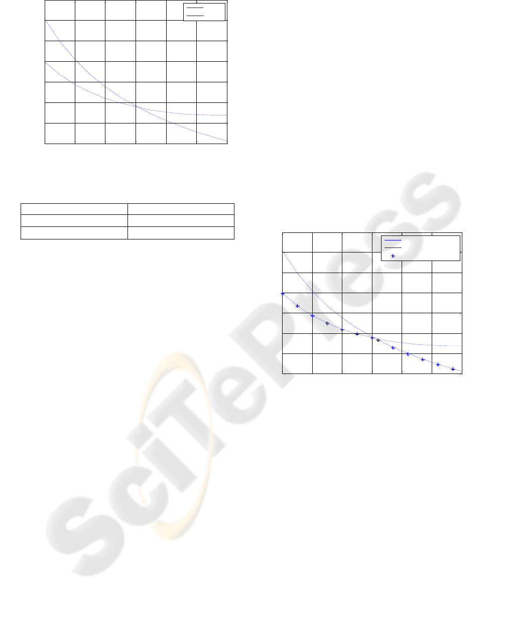
Figure 4: The energy consumptions for GBR and GBR-C.
Table 2: Next hop nodes number.
Transmission Probability
Next Hop Nodes Number
n=1 GBR
n=2 GBR-C
4.3 Auto-adaptable GBR-C Protocol
In the former section, it was concluded that GBR-C
has the potential of saving energy when the
transmission probability P is less than a certain
threshold. However, in real networks, sometimes it
is hard to know the value of P before networks are
deployed. To over come this, in this section, an
algorithm is proposed which can make nodes adapt
their next hop nodes numbers automatically
according to the transmission probability P. The new
protocol with this algorithm is referred to as auto-
adaptable GBR-C protocol.
The main idea of this algorithm is to keep
calculating the real time transmission probability.
For a reliable communication model, every sender
will wait for an ACK message after it sends a data
message. So the transmission probability can be
obtained by recording the send number and the ACK
number. Firstly, variables used to record numbers
which will be used to calculate the transmission
probability are defined.
Sn is used to record the number of the data
message that this node has already sent.
Rn is used to record the number of the ACK or
DACK message that this node has already received.
P refers to the real time transmission probability
that we are looking for.
The details of this algorithm are as follows:
1) p is initialized as one.
2) Each node checks the value of p before it
sends a data message. If p is less than the
threshold (p=0.71), then this node sets two
next hop destination nodes for this data
message, otherwise it sets one.
3) Sn will be increased when the node sends a
data message. Sn will be increased by 1 if
this data message has only one next hop
destination node. It will be increased by 2 if
this data message has 2 next hop destination
nodes.
4) Then, the node will wait for the ACK or
DACK message and Rn will be increased
by 1 when the node has received an ACK or
DACK message.
5) The node calculates its transmission
probability by the equation P=Rn/Sn, and
then returns to step 2).
The energy consumption that is obtained for the
auto-adaptable GBR-C protocol is shown in Figure
5.
Figure 5: The energy consumption for auto-adaptable
GBR-C.
5 SIMULATION & RESULTS
The competing algorithm protocols GBR-C and
auto-adaptable GBR-C were implemented in the
Omnet++ network simulator. The results obtained
were compared with the GBR protocol.
5.1 Simulation Configurations
In our simulations, two wireless sensor networks
were considered. One is a regular network which is
shown in Figure 6 (a) with 11 static sensor nodes
deployed inside a rectangle field regularly with one
sink and one source. The other one is a random
network shown in Figure 6 (b) with 50 static sensor
nodes deployed inside a rectangle field randomly
0.4 0.5 0.6 0.7 0.8 0.9 1
4
5
6
7
8
9
10
11
P
Energy (mw)
GBR
GBR-C
0.4 0.5 0.6 0.7 0.8 0.9 1
4
5
6
7
8
9
10
11
P
Energy (mw)
GBR
GBR-C
Auto-adaptable GBR-C
WINSYS 2010 - International Conference on Wireless Information Networks and Systems
86
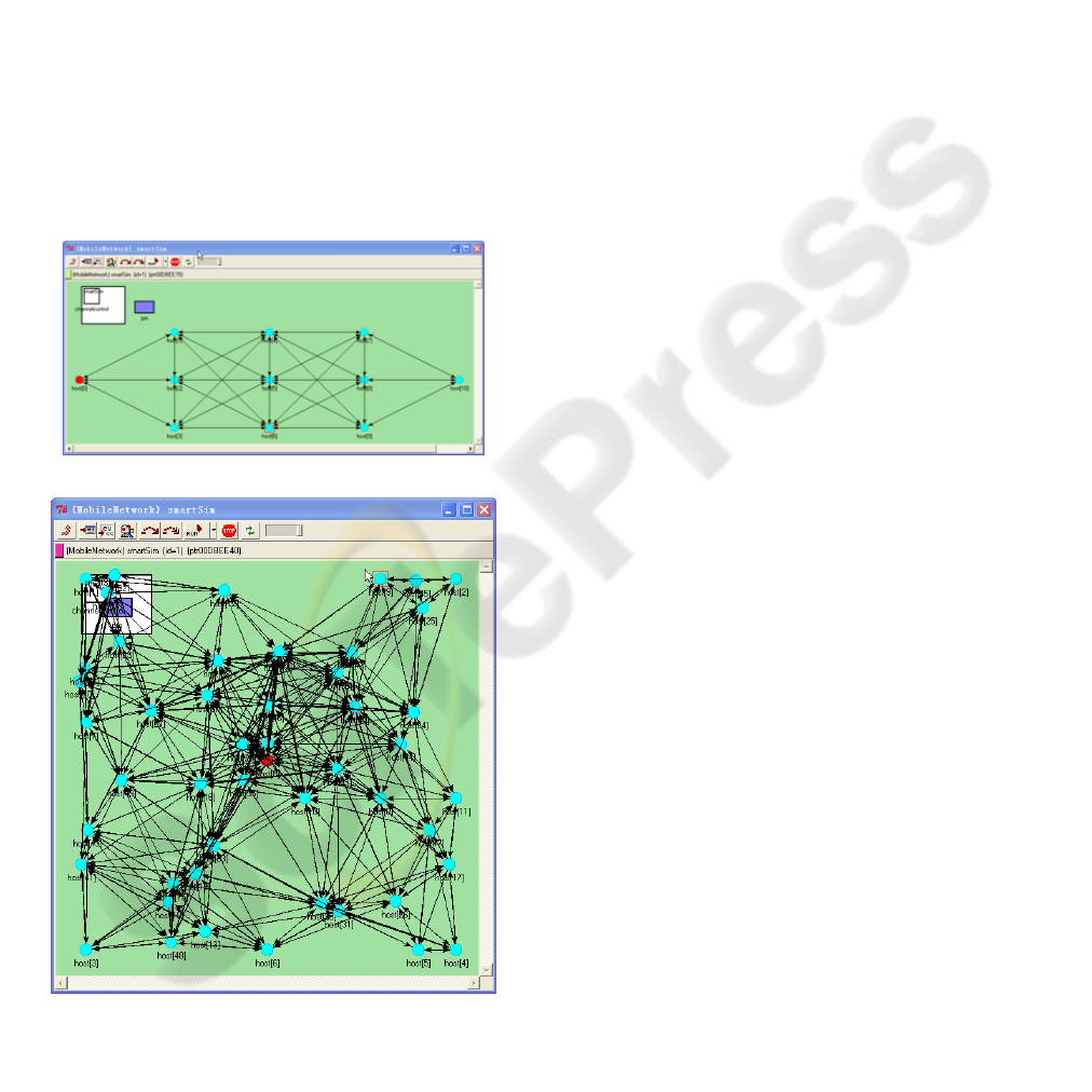
with one sink and four sources. For the regular
network, each node has a fixed radio range of 300
meters. For the random network, each node has a
fixed radio range of 200 meters. The positions of the
sources and sinks are shown in Figure 6. In these
configurations, the sinks and sources are located far
from each other which facilitate the evaluation of the
protocol where the routing path has to traverse a
large area in the sensor field.
The EnergyFramework-2.0 provided in the
Omnet++ is used and each node is assigned with the
same initial energy capacity of 40 J at the beginning
of each simulation. The energy consumption is
further set for sending time and receiving time as
65mw/sec and 21mw/sec respectively (The same
parameters as Mica2 power consumption model). In
addition, W. Ye, et al., (2002) have showed that
compared to sending and receiving, the sleeping
time consumption is very small. As a result, the
SINK SOURCE
(a)
SINK
SOURCESOURCE
SOURCE SOURCE
(b)
Figure 6: The simulation networks: (a) Regular wireless
sensor network; (b) Random wireless sensor network.
sleeping time energy consumption is ignored and set
to 0. The B-MAC layer (Joseph Polastre, et al., 2004)
is used, the MAC bit rate and the messages length
are set as same as in Section 3. The simulation steps
are as follows:
1) Sinks broadcast interest message through
the whole network, and the interest will be
resent every 1500 seconds.
2) Sources gather and sends data to the sinks
every 30 seconds.
3) Stop simulating when the sink has received
a certain number (300 for regular network,
1000 for random network) of messages
from sources.
4) Output the simulation data.
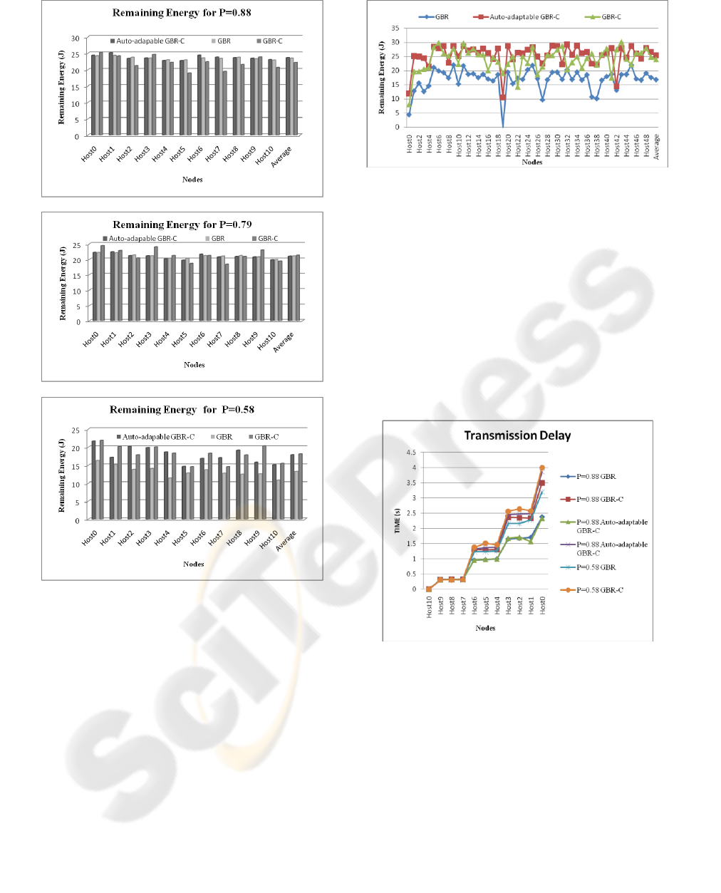
5.2 Results and Discussion
Figure 7 shows the remaining energy for the regular
network after the simulation under different
transmission probability setting. Here the probability
is set by dropping a certain percent packet, such as
p=0.88 which means 12% messages is dropped by
each node. It can be observed that GBR-C uses less
energy than GBR to deliver the same number of
messages when the transmission probability p less
than 0.79 which verifies the conclusion that GBR-C
has the potential to save energy when the probability
P is less than a certain threshold. Compared to GBR,
GBR-C can save up to 18% energy when p=0.58 for
4 hops transmission. However, the simulation result
shows that the threshold is p=0.79 and it is a little
higher than 0.71 which was obtained in Section 4.2.
In this simulation, as well as in some real networks,
the messages will be dropped after three failure
transmissions. GBR-C chooses one more next hop
nodes to transmit the message which can reduce the
number of dropped messages in the intermediate
nodes. As a result, in a real network, it is shown that
the GBR-C can save more energy than in theory.
This is why the simulation threshold value is 0.79
which is greater than the theoretic value 0.71.
Figure 7 also shows that the auto-adaptable
GBR-C is like GBR when p=0.88 which is greater
than the threshold P=0.71 and is like GBR-C when
p=0.58 which is less than the threshold. The
simulation results showed that for all network
environments, the auto-adaptable GBR-C performed
better in terms of energy efficiency.
A COMPETING ALGORITHM FOR GRADIENT BASED ROUTING PROTOCOL IN WIRELESS SENSOR
NETWORKS
87
(a)
(b)
(c)
Figure 7: The remaining energy histogram for regular
network with different transmission probability: (a)
p=0.88 (b) p=0. 79 (c) p=0.58.
Figure 8 shows the remaining energy for the
random network after the simulation. In this
network, the transmission probability for each node
is, the average transmission probability
for the whole network is p=0.63.It can be observed
that the auto-adaptable GBR-C performs better in
terms of energy efficiency for this random wireless
sensor network.
Figure 9 shows the average transmission delays
for the regular network under different transmission
probability. It can be observed that GBR-C has a
little longer delay than GBR. This is because GBR-C
uses the competing algorithm for every hop
Figure 8: The remaining energy for random network.
transmission and needs to wait for the TOGO
message before sending the message. For the auto-
adaptable GBR-C, the transmission delay is close to
GBR when p is greater than the threshold and close
to GBR-C when p is less than the threshold. It also
can be observed that the delay of GBR increases
faster then GBR-C when p decrease. This is because
that GBR-C reduces the probability of
retransmission and saves retransmission delay.
Herewith, the delay of GBR-C could shorter than
GBR with a certain p and a short waiting time for
TOGO.
Figure 9: The transmission delay.
6 CONCLUSIONS
In this paper, a competing algorithm for GBR in
wireless sensor networks was proposed.
Furthermore, an Auto-adaptable GBR-C routing
protocol for wireless sensor networks was proposed.
The competing algorithm aims to reduce the
retransmission attempts and save the energy by
considering two next hop nodes. Simulation results
showed that the proposed scheme has higher energy
efficiency than the GBR, but with a little longer
WINSYS 2010 - International Conference on Wireless Information Networks and Systems
88

transmission delay. In the future, studies will be
carried out to find transmission probability threshold
more accurately and to reduce the transmission delay.
ACKNOWLEDGEMENTS
The authors would like to thank F’SATI at Tshwane
University of Technology and Telkom Centre of
Excellence program for making this research
possible.
REFERENCES
C. Schurgers and M. B. Srivastava, 2001. Energy efficient
routing in wireless sensor networks. In the MILCOM
Proceedings on Communications for Network-Centric
Operations: Creating the Information Force, McLean,
VA.
Al-Karaki, J. N and Kamal, A.E, 2004. “Routing
techniques in wireless sensor networks: a survey.” In
the Wireless Communications, IEEE:, page(s): 6- 28.
Shnayder, V., Hempstead, M., Chen, B., Allen, G. W., and
Welsh, M., 2004. “Simulating the power consumption
of large-scale sensor network applications.” In
Proceedings of the 2nd international Conference on
Embedded Networked Sensor Systems (Baltimore,
MD, USA).
W. Ye, J. Heidemann, and D. Estrin., 2002 . “An Energy-
Efficient MAC Protocol for Wireless Sensor
Networks.” In Proceedings of the 21st International
Annual Joint Conference of the IEEE Computer and
Communica.
Joseph Polastre, Jason` Hill, David Culler, 2004.
“Versatile Low Power Media Access for Wireless
Sensor Networks,” ACM Sensys.
H. Fussler, J. Widmer, M. Kasemann, M. Mauve, and H.
Hartenstein, 2003. “Contention-based forwarding for
mobile ad-hoc networks,” Elsevier’s Ad Hoc
Networks, vol. 1, no. 4, pp. 351–369.
M. Zorzi and R. R. Rao, 2003. “Geographic random
forwarding (geraf) for ad hoc and sensor networks:
energy and latency performance,” IEEE.
S. Biswas and R. Morris, 2005. “Exor: Opportunistic
multi-hop routing for wireless networks,” in
SIGCOMM’05, Philadelphia, Pennsylvania.
K. Zeng, W. Lou, and H. Zhai, 2008. "On end-to-end
throughput of opportunistic routing in multirate and
multihop wireless networks," in Proceedings of the
Annual Joint Conference of the IEEE Computer and
Communications Societies (INFOCOM '08), pp. 1490-
1498, Phoenix, Ariz, USA.
K. Zeng, W. Lou, J. Yang and D. Brown, 2007. “On
geographic collaborative forwarding in wireless ad hoc
and sensor networks,” in WASA’07, Chicago, IL.
A COMPETING ALGORITHM FOR GRADIENT BASED ROUTING PROTOCOL IN WIRELESS SENSOR
NETWORKS
89
