Automatic Modularization of Artificial Neural Networks
Eva Volna
University of Ostrava, 30
ht
dubna st. 22, 701 03 Ostrava, Czech Republic
Abstract. The majority of this paper relies on some forms of automatic decom-
position tasks into modules. Both described methods execute automatic neural
network modularization. Modules in neural networks emerge; we do not build
them straightforward by penalizing interference between modules. The concept
of emergence takes an important role in the study of the design of neural net-
works. In the paper, we study an emergence of modular connectionist architec-
ture of neural networks, in which networks composing the architecture compete
to learn the training patterns directly from the interaction of reproduction with
the task environment. Network architectures emerge from an initial set of ran-
domly connected networks. In this way can be eliminated connections so as to
dedicate different portions of the system to learn different tasks. Mentioned me-
thods were demonstrated for experimental task solving.
1 Reasons for a Modular Approach
The primary reason for adopting an ensemble approach to combining nets into a
modular architecture is that of improving performance. There are a number of possi-
ble justifications for taking a modular approach to combining artificial neural nets.
First, a modular approach might be used to solve a problem which could not have
been solved through the use of a unitary net. A modular system of nets can exploit the
specialist capabilities of the modules, and consequently achieve results, which would
not be possible in a single net. Another reason for adopting a modular approach is
that of reducing model complexity, and making the overall system easier to under-
stand. This justification is often common to engineering design in general. Other
possible reasons include the incorporation of prior knowledge, which usually takes
the form of suggesting an appropriate decomposition of the global task. A modular
approach can also reduce training times and make subsequent modification and ex-
tension easier. Finally, a modular approach is likely to be adopted when there is con-
cern to achieve some degree of neurobiological or psychological plausibility, since it
is reasonable to suppose that most aspects of information processing involve mod-
ularity.
A modular neural network can be characterized by a series of independent neural
networks moderated by some intermediary. Each independent neural network serves
as a module and operates on separate inputs to accomplish some subtask of the task
the network hopes to perform [1]. The intermediary takes the outputs of each module
and processes them to produce the output of the network as a whole. The interme-
Volna E. (2010).
Automatic Modularization of Artificial Neural Networks .
In Proceedings of the 6th International Workshop on Artificial Neural Networks and Intelligent Information Processing, pages 23-32
Copyright
c
 SciTePress

seen in terms of the backpropagation algorithm, it is limited to networks trained using
this algorithm. Therefore, spatial crosstalk may be considered as resulting from the
connectivity of the network and not from the learning algorithm used to training the
network. By maintaining short connections and eliminating long connections, spatial
crosstalk can be reduced and tasks can be decomposed into subtasks. Although the
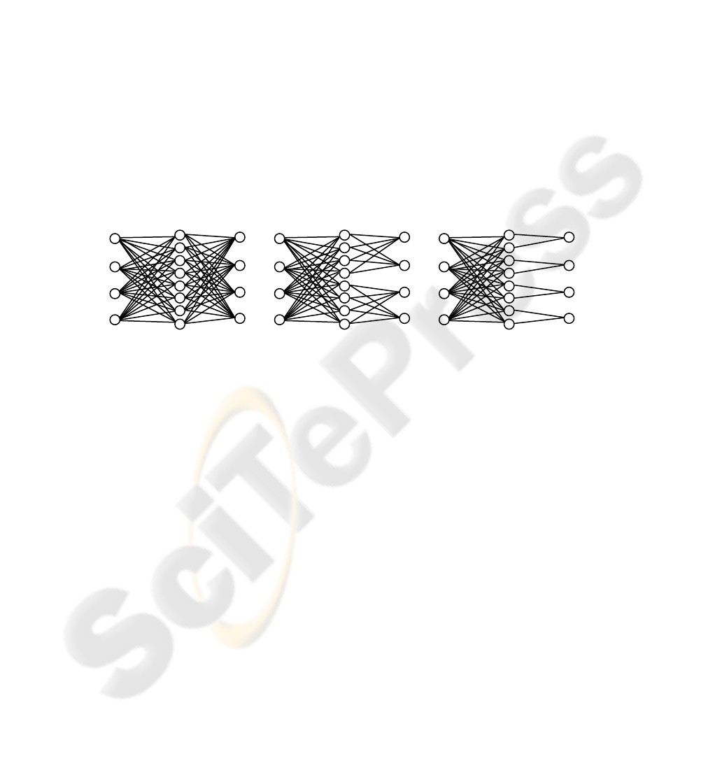
three systems show in Fig. 1 [5] can be trained to perform the same mapping. System
in Panel A has its hidden units fully interconnected with its output units and is most
susceptible to spatial crosstalk. System in the Panel B has its hidden units on the top
fully interconnected with its top output units and its hidden units on the bottom fully
interconnected with its bottom output units. Thus, it consists of two separate networks
(two 4-4-2 networks). If the mapping that this system is trained to perform can be
decomposed so that the mapping from the input units to the top set of output units
may be thought of as one task and the mapping from the input units to the bottom set
of output units may be thought of as a second task, then this system has dedicated
different networks to learn the different tasks. Because there is no spatial crosstalk
between the two tasks, such a system may show rapid learning. The Panel C has hid-
den unit project to only a single output unit. It therefore consists of a separate net-
work for each output unit (four 4-2-1 networks) and is immune to spatial crosstalk.
A B C
Fig. 1. A: One 4-8-4 network. B: Two 4-4-2 networks. C: Four 4-2-1 networks [5].
Artificial neural network with many adjustable weights may learn to training data
quickly and accurately, but generalize poorly to novel data. One method of improving
the generalization abilities of network with too many “degrees of freedom” is to de-
cay or eliminate weights during training. A second method is to match the structure of
the network with the structure task. For example, networks, whose units have local
receptive fields, can learn to reliably, detect the local structure that is often present in
pattern recognition tasks. A system that maintains short connections and eliminates
long connections should generalize well because its degrees of freedom are reduced
and because its units develop local receptive fields.
Artificial neural network often develop relatively not interpretable representations
for at least two reasons. Networks whose units are densely connected tend to develop
representations that are distributed over many units and, thus, are difficult to interpret.
In addition, not interpretable representations often develop in networks that are
trained to simultaneously perform multiple tasks. In contrast, networks, whose units
tend to have local receptive fields, towards short connections may develop relatively
local representations. Furthermore, such a system may be capable of eliminating
connections so that different networks learn different tasks.
25

3 Evolutionary Module Acquisition
There is a simple model of evolutionary emergence of modular neural network topol-
ogy introduced in the chapter [10]. We describe a method of optimization of the
modular neural network architecture via evolutionary algorithms that uses a fix part
of network architecture in the genome. Every individual is a multilayer neural net-
work with one hidden layer of units. We have to fix its maximal architecture (e.g.
number of input, hidden and output units) before the main calculation. Population P
consists of P = {
α 1, α 2,..., α p}, where p is equal to a number of chromosomes in P.
Every chromosome consists of binary digits that are generated randomly with a prob-
ability 0.5. Chromosome, with m hidden units a n output units is shown in Fig. 2,
where e
ij = 0, if the connection between i - th hidden unit and j - th output unit of the
individual doesn’t exist, and eij = 1, if the connection exists (i = 1,…,m; j = 1,…n).
Connections between input and hidden units are not included in chromosomes, be-
cause they are not necessary for modular network architecture creation. Each individ-
ual (e.g. the network architecture) is partially adapted by backpropagation, its fitness
function is then calculated as follows (1):
k
k
E
Fitness
1
=
(1)
where k = 1, …, p (p = number of individuals in the population);
k
E is the error after backpropagation adaptation of the k-individual.
Population P:
individual:
α
1
...
individual: α
k
...
individual: α
p
INDIVIUAL
α
k
:
e
11
, …e
1n
, ... e
m1
, …e
mn
Fig. 2. A population of individuals.
Only two mutation operators are used, no crossover operators. The first mutation
operator is defined in following way. In the every generation, one individual is ran-
domly chosen and each bit is changed with probability 0.01 (e.g. if the connection
exists – after mutation it does not exist and vice versa) in its chromosome. The
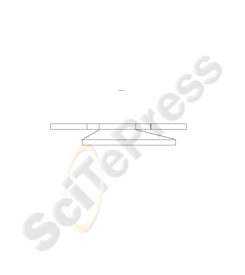
second mutation operator is defined in following way, see Fig. 3. First, we define a
pattern of t-consecutive zeroes that will be fixed during whole calculation. The pat-
tern is determined by number of neurons in the output layer, which represent individ-
ual modules. Output neurons are organized into d modules, t = min (t
i, i = 1 ,..., d),
where t is number of neurons in the pattern, and ti is number of neurons in the i-th
module. Defined pattern is represented as a continuous chain of t-zeros, which is not
changed during applications of the second mutation operator. Fixation of t-zeros
chain can be defended by biological motivation, where the protection against muta-
tion is usually related to continuous section. Defined pattern in the chromosome al-
lows temporary fixing the existing module against the application of the second muta-
tion operator. Then we find the define pattern in each chromosome. If we find only
26

one continuous pattern, we fix it. If we find more than n-consecutive zeroes, we ran-
domly choose n-consecutive zeroes from them and fix them. The fixed pattern
represents a single atomic unit and the second mutation operator is not applied to it.
Only to the rest of bits from chromosomes are changed with probability 0.01. Thus,
each individual has a unique collection of fixed patterns. The second mutation opera-
tor is applied to every individual r - times, where r is a parameter and its value is
define before calculation. Only the best individual or its best mutation is included into
the next generation. Next, all individuals in the new generation release a portion of
the pattern that was fixed that way they can once again be manipulated by reproduc-
tion operators. The process of evolutionary algorithms
is ended when the population
achieves the maximal generation or if there is no improvement in the objective func-
tion for a define sequence of consecutive generations.
00...0000010...
A
:
B:
00100010101
0...0
110010
0...0
k < t k = t k > t
00100010101
0...0
1100100...00
0...0
000010...
00100010101
0...0
1100100..
.000.
..0000010...
Fig. 3. The second mutation operator. The fixed pattern is t- consecutive zeroes, k is number of
consecutive zeroes in the chromosome. A: An individual before mutation. B: Possible chromo-
somal representation of the individual after mutation.
4 Modularization Via Evolutionary Hill – climbing Algorithm
The second presented method is based on hill-climbing algorithm with learning [8].
Evolution of the probability vector is modeled by a genetic algorithm on the basis of
the best evaluated individuals in this algorithm, which are selected on the basis of the
speed and quality of learning of the given tasks [11]. Population P is presented in Fig.
2 and is defined in the same way as in the previous chapter. Individuals in the next
generation are generated from the updating probability vector. Every individual (e.g.
its neural network architecture) is partially adapted by backpropagation [2] and eva-
luated by the quality of its adaptation. The number of epochs is a very important
criterion in the described method, because modular architectures start to learn faster
than fully connected multilayer connectionist networks [9]. Our goal is to produce
such a neural network architecture that is able to learn a given problem with the smal-
lest error. A backpropagation error is a fitness function parameter. A fitness function
value F
i of the i - th individual is calculated as follows (2):
con
f
F
con
k
ik
i
∑
=
=
1
(2)
where i = 1, …, p (p is number of individuals in a population);
27

The best individual in the population is included to the next population automati-
cally. Values of the chromosomes of the rest of individuals
α i (i = 2, …,p) are calcu-
lated for the next generation as follows: if wk = 0(1), then (ek)i = 0(1); if 0 < wk < 1
the corresponding (ek)i is determined randomly by (6):
()
⎩
⎨
⎧
<
=
otherwise0
i1
k
i
k
wrandomf
e
(6)
where k = 1, …, p (p = number of individuals in the population).
The process of the evolutionary algorithm is ended if the saturation parameter
τ (w)
*
is greater than a predefined value.
5 Experiments
In the experimental task, a system (neural network) recognizes a binary pattern and
its rotation. Neural network with one hidden layer of units with topology 9-13-8
adapted by backpropagation represents a system here. The creation of such modular
system that would solve partial tasks correctly was our target. Basic set of training
patterns are organized into a matrix (grid) 3x3, which is represented by binary vector.
The direction of rotation is defined towards the basic pattern by four possibilities: (a)
0°-state without rotation, (b) turn 90°, (c) turn 180°, and (d) turn 270°. The training
set includes four patterns that are defined in four different states, see Fig 4. Thus, we
get 16 different combinations of shapes and their rotations. Eight output units are
divided into two subsets of four units. Units in the “shape” subset are responsible for
indicating the identity of the input. Each input is associated with one of the four
“shape” units, and one of the four rotations. The system is considered to correctly
recognize and locate an input.
Parameters of the Experimental part.
− Population (both methods):
Number of individuals: 100.
Neural network architecture: 9 – 13 – 8.
Training algorithm: Backpropagation
(learning rate: 1; momentum: 0; training times: 150 epochs in the partial training).
− Parameters of method from chapter 3:
Probability of mutations: 0.01.
Fix pattern in the second mutation: “0000”.
r: 5.
Ending conditions: Maximal number of generations: 500.
*
τ (w) = a number of entries (wi) of the probability vector w that are less then weff or (1- weff),
where weff is a small positive number.
29

− Parameters of method from chapter 4:
con: 100; see formula (2).
λ : 0.2; see formula (4).
Ending conditions: The saturation parameter,
τ (w): 0.99*m*n
(m=13, number of hidden units; n=8, number of output units); weff = 0.01.
Fig. 4. A defined pattern in a training set.
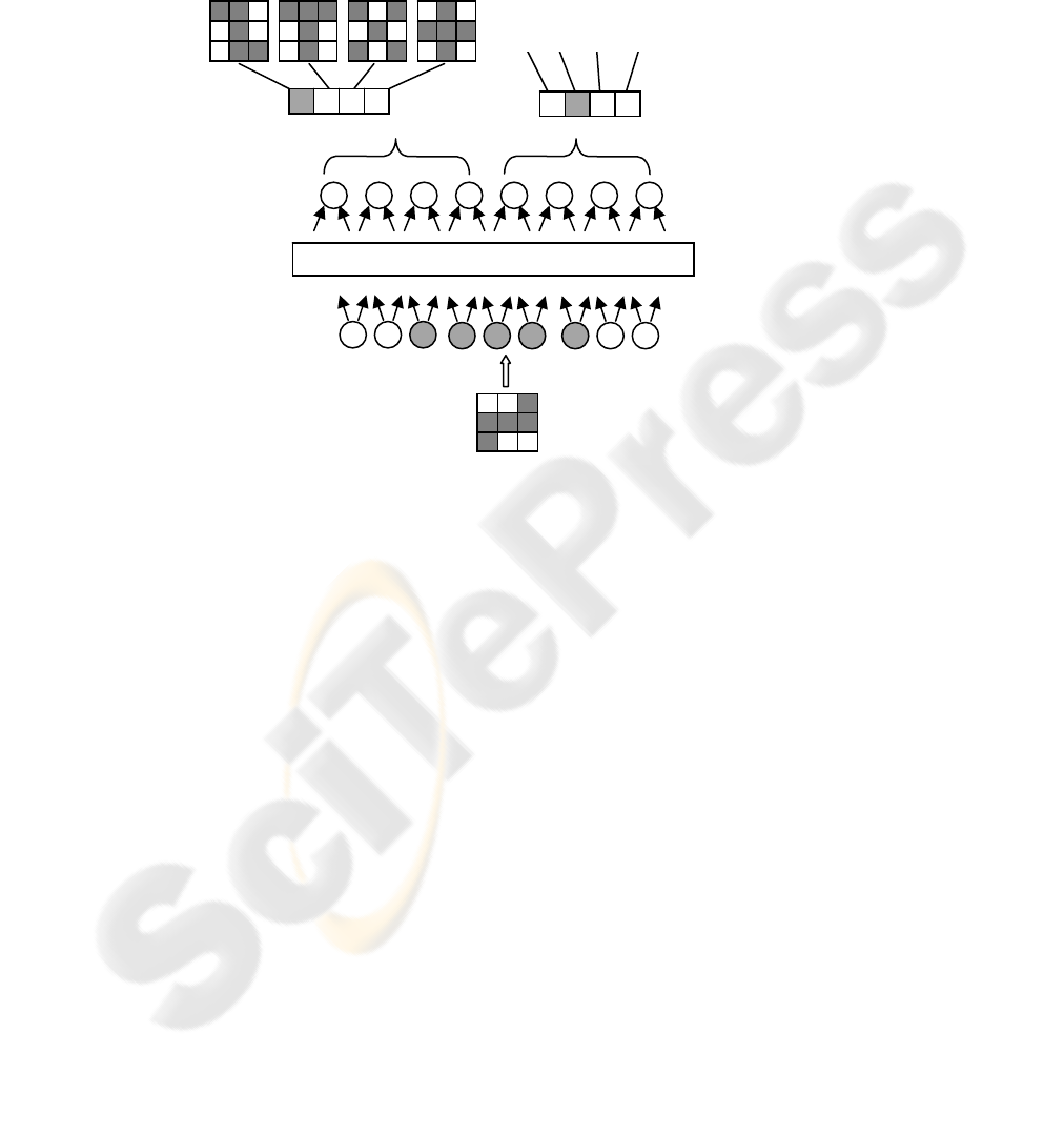
Table 1 shows a table of results. The table shows an evolution of the best individ-
ual in the population. It is evidently seen, the connections among modules are elimi-
nated faster than connection inside modules. These results support also the fact that
systems were created dynamically during a learning process. Method from chapter 3
gives the following results: six hidden units of the best individual realise the “shape”
task and its four units realise the “rotation” task in the last generation. Method from
chapter 4 gives the following results: seven hidden units of the best individual realise
the “shape” task and its four units realise the “rotation” task in the last generation.
Calculation was terminated, when ending conditions were fulfilled, e.g. for method
from chapter 3 was calculation terminated in the 498-th generation and for method
from chapter 4 was calculation terminated in the 353-rd generation. Other numerical
simulations give very similar results.
Table 1. Table of results.
OUTPUT
WHICH SHAPE
SHAPE ROTATION
I
NPUT
HIDDE
N
LAYER
0°
90°
180°
270°
IN
P
U
T
: s
h
ape
1
,
r
otat
i
o
n
90
°
30

Method from chapter 3: Method from chapter 4:
generation
number of
hidden
units:
„shape“
task:
number of
hidden units:
„rotate“
task:
number of
interferen-
ces:
number of
hidden units:
„shape“
task:
number of
hidden units:
„rotate“
task:
number of
interferen-
ces:
1 1 1 11 0 0 13
100 2 3 8 1 3 9
200 3 3 7 4 3 6
300 4 3 6 6 3 4
400 5 4 4 GENERATION: 353
GENERATION: 498 7 4 2
6 4 3
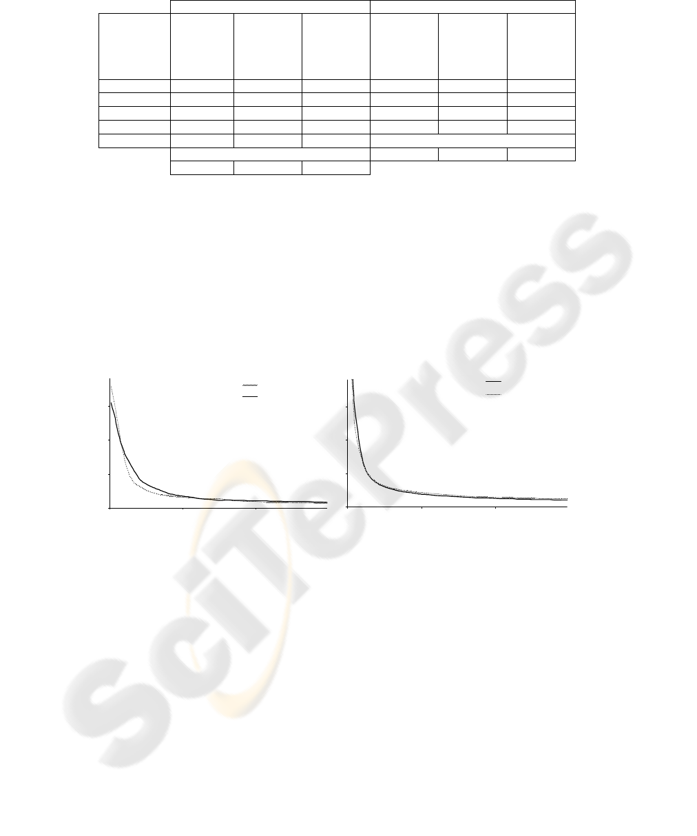
We made the following experiment. Neural network with modular architecture (the
best individual) and network with the same arrangement of neurons, but by all con-
nections between layers have been adapted via backpropagation to solve the above
defined task. For each model was done 10 adaptations, the weight vector was at the
beginning of each simulation generated randomly. In Fig. 5 the average error function
values is shown: (a) modular neural network and (b) fully connected neural network
during the whole calculation. Adaptation of each neural network was terminated after
1500 iterations. The figure shows that the network with a modular architecture, which
includes only a limited number of connections, allows to learn the considered prob-
lem as efficiently as a monolithic networks designed within an appropriate architec-
ture.
0
5
10
15
0 500 1000
fully connected individual
modular architecture
iter ations
E
0
5
10
15
0 500 1000
modular architecture
fully connected individual
iter ati ons
E
A B
Fig. 5. The history of average error function value during whole calculation A: method from
chapter 3; B: method from chapter 4.
6 Conclusions
Both described method are methods of automatic neural net modularization. The
problem specific modularisations of the representation emerge through the iteration
of the evolutionary algorithm directly with the problem.
When interpreting solutions, we have to be careful, because algorithms’ parame-
ters are not the object of the optimization process, but we obtain solutions just in
dependence on these parameters. Both numerical simulations reflect the modular
31

structure significance as a tool of a negative influence interference rejection on neural
network adaptation. As the hidden units in the not split network are perceived as
some input information processing for output units, where a multiple pattern classifi-
cation is realized on the basis of diametrically distinct criteria (e.g. neural network
has to classify patterns according to their form, location, colors, ...), so in the begin-
ning of an adaptation process the interference can be the reason that output units also
get further information about general object classifications than the one which is
desired from them. This negative interference influence on running the adaptive
process is removed just at the modular neural network architecture, which is proved
also by results of the performed experiment. The winning modular network architec-
ture was the product of emergence using evolutional algorithms. The neural network
serves here as a special way of solving the evolutional algorithm, because of its struc-
ture and properties it can be slightly transformed into an individual in evolutionary
algorithm.
References
1. Di Fernando, A., Calebretta, R., and Parisi, D. (2001) Evolving modular architectures for
neural networks. In French R., and Sougne, J. (eds.).Proceedings of the Sixth Neural Com-
putation and Psychology Workshop: Evolution, Learning and Development. Springer Ver-
lag, London.
2. Fausett, L. V. (1994) Fundamentals of neural networks. Prentice-Hall, Inc., Englewood
Cliffs, New Jersey.
3. Hampshire, J. and Waibel, A. The Meta-Pi network: Building distributed knowledge repre-
sentation for robust pattern recognition. Technical Report CMU-CS-89-166. Pittsburgh,
PA: Carnegie Mellon University.
4. Jacobs, R. A., Jordan, M. I., Nowlan, S.J., and Hinton, G. E. (1991) Adaptive mixtures of
local experts. Neural Computation, 3, pp.79-97.
5. Jacobs, R. A., Jordan, M. I. (1992). Computational consequences of a bias toward short
connections. Journal of Cognitive Neuroscience, 4, 323–336.
6. Jacobs, R. A. (1994) Hierarchical mixtures of experts and the EM algorithm. Neural Com-
putation, 6, 181-214.
7. Jordan, M. I. and Jacobs, R. A. (1995) Modular and Hierarchical Learning Systems. In M.
A. Arbib (Ed) The Handbook of Brain Theory and Neural Networks. pp 579-581.
8. Kvasnička, V; Pelikán, M.; Pospíchal, J. (1996) Hill climbing with learning (an abstraction
of genetic algorithm). Neural network world 5, 773-796.
9. Rueckl, J. G. (1989) Why are “What” and “Where” processed by separate cortical visual
systems? A computational investigation. Journal of Cognitive Neuroscience 2, 171-186.
10. Volna, E. (2002) Neural structure as a modular developmental system. In P. Sinčák, J.
Vaščák, V. Kvasnička, J. Pospíchal (eds.): Intelligent technologies – theory and applica-
tions. IOS Press, Amsterdam, pp.55-60.
11. Volna, E. (2007) Designing Modular Artificial Neural Network through Evolution. In J.
Marques de Sá, L. A. Alexandre, W. Duch, and D. P.Mandic (eds.) Artificial Neural Net-
works – ICANN’07, Lecture Notes in Computer Science, vol. 4668, Springer-Verlag series,
pp 299-308.
32