Feature Transformation and Reduction
for Text Classification
Artur J. Ferreira
1,3
and M´ario A. T. Figueiredo
2,3
1
Instituto Superior de Engenharia de Lisboa, Lisboa, Portugal
2
Instituto Superior T´ecnico, Lisboa, Portugal
3
Instituto de Telecomunicac¸˜oes, Lisboa, Portugal
Abstract. Text classification is an important tool for many applications, in su-
pervised, semi-supervised, and unsupervised scenarios. In order to be processed
by machine learning methods, a text (document) is usually represented as a bag-
of-words (BoW). A BoW is a large vector of features (usually stored as floating
point values), which represent the relative frequency of occurrence of a given
word/term in each document. Typically, we have a large number of features, many
of which may be non-informative for classification tasks and thus the need for
feature transformation, reduction, and selection arises. In this paper, we propose
two efficient algorithms for feature transformation and reduction for BoW-like
representations. The proposed algorithms rely on simple statistical analysis of
the input pattern, exploiting the BoW and its binary version. The algorithms are
evaluated with support vector machine (SVM) and AdaBoost classifiers on stan-
dard benchmark datasets. The experimental results show the adequacy of the re-
duced/transformed binary features for text classification problems as well as the
improvement on the test set error rate, using the proposed methods.
1 Introduction
In text classification tasks, each document is typically represented by a bag-of-words
(BoW) or similar representation. A BoW is a high-dimensional vector with the rela-
tive frequencies of a set of terms in each document. A collection of documents is usu-
ally represented by the term-document (TD) [13] matrix whose columns hold the BoW
representation for each document whereas its rows correspond to the terms in the col-
lection. An alternative representation for a collection of documents is provided by the
(binary) term-document incidence (TDI) matrix [13]; this matrix holds the information,
for each document, if a given term (word) is present or absent.
For both the TD or TDI matrix, we usually have a large number of terms (features),
many of which are irrelevant (or even harmful) for the classification task of interest.
On the other hand, this excessive number of features carries the problem of memory
usage in order to represent a large collection of documents and to allow efficient queries
on a database of documents. This clearly shows the need for feature transformation,
reduction, and selection, to both improve the classification accuracy and the memory
requirements. We are thus lead to a central problem in machine learning: choosing the
J. Ferreira A. and Figueiredo M.
Feature Transformation and Reduction for Text Classification.
DOI: 10.5220/0003028100720081
In Proceedings of the 10th International Workshop on Pattern Recognition in Information Systems (ICEIS 2010), page
ISBN: 978-989-8425-14-0
Copyright
c
 2010 by SCITEPRESS – Science and Technology Publications, Lda. All rights reserved

most adequate set of features for a given problem. There are many feature selection and
reduction techniques in the literature; a comprehensive listing of these techniques is too
extensive to be presented here (see for instance [4, 8,9]).
For text classification tasks, several techniques have been proposed for feature re-
duction (FR) and feature selection (FS) [6,10,14,16]. The majority of these techniques
is applied directly on BoW representations (TD matrix).
1.1 Our Contribution
In this paper, we propose two methods for FS in text classification problems using
the TD and the TDI matrices. These methods do not tied to the type of classifier to
be used; one of the methods does not use the class label, thus being equally suited
for supervised, semi-supervised, and unsupervised learning. As shown experimentally,
the proposed methods significantly reduce the dimension of the BoW datasets, while
improving classification accuracy, as compared to the classifiers trained on the original
features.
The remaining text is organized as follows. Section 2 briefly reviews the basic con-
cepts regarding BoW representations, SVM, and AdaBoost classifiers. Section 3 de-
scribes the proposed methods and Section 4 presents experimental results on standard
benchmark datasets. Finally, Section 5 ends the paper with some concluding remarks.
2 Background
Text classification and categorization arises in many information retrieval (IR) appli-
cations [13]. As the size of the datasets on which IR is performed rapidly increases, it
becomes necessary to use strategies to reduce the computational effort (i.e. time) to per-
form the necessary searches. In many applications, the representation of text documents
typically demands large amounts of memory. As detailed in the following subsections,
some classification tools (namely SVM and AdaBoost) have been proven effective for
text classification with BoW representations, whereas other techniques that perform
well in other types of problems show more modest results when used for text classifi-
cation.
2.1 Bag-of-Words (BoW) and Support Vector Machines (SVM)
A BoW representation consists in a high-dimensional vector containing some measure,
such as the term-frequency (TF) or the term-frequency inverse-document-frequency
(TF-IDF) of a term (or word) [11] in a given document. Each document is represented
by a single vector, which is usually sparse, since many of its features are zero [11]. The
support vector machine (SVM) [17] classifier works in a discriminative approach, by
finding the hyperplane that separates the training data with maximal margin. The SVM
has been found very effective for BoW-based text classification [3,6,11,16]. In this
paper, we apply SVM classifiers on original and reduced BoW representations in order
to evaluate the performance of the proposed FS methods.
73

2.2 The AdaBoost Algorithm
The AdaBoost algorithm [7,9] learns a combination of the output of M (weak) classi-
fiers G
m
(x) to produce the binary classification (in {−1, +1}) of pattern x, as
G(x) = sign
M
X
m=1
α
m
G
m
(x)
!
, (1)
where α
m
is the weight (which can be understood as a degree of confidence) of each
classifier. The weak classifiers are trained sequentially, with a weight distribution over
the training set patterns being updated in each iteration according to the accuracy of
classification of the previous classifiers. The weight of the misclassified patterns is in-
creased for the next iteration, whereas the weight of the correctly classified patterns is
decreased. The next classifier is trained with a re-weighted distribution. The AdaBoost
algorithm (and other variantsof boosting) has been successfully applied to several prob-
lems, but regarding text classification there is no evidence of performance similar to the
one obtained with SVM [3,15].
3 Proposed Methods
In this section, we describe the proposed methods for FS to be used in text classification.
Let D = {(x
1
, c
1
), ..., (x
n
, c
n
)} be a labeled dataset with training and test subsets,
where x
i
∈ R
p
denotes the i-th (BoW-like) feature vector and c
i
∈ {−1, +1} is the
corresponding class label. Let X be the p × n TD matrix corresponding to D, i.e., the
i-th column of X contains x
i
, whereas each row corresponds to a term (e.g. word).
Let X
b
be the corresponding (binary) p×n TDI matrix, obtained from X according
to
X
b
(t, d) =

0 ⇐ X(t, d) = 0,
1 ⇐ X(t, d) 6= 0,
(2)
for t ∈ {1, . . . , p} and d ∈ {1, . . . , n}.
The proposed methods for FS rely on a simple sparsity analysis of the TD or TDI
matrix of the training set, using the ℓ
0
norm (the number of non-zero entries); these
methods compute the ℓ
0
norm of each feature (i.e., each row of X or X
b
).
3.1 Method 1 for Feature Selection
Given an p×n TD matrix X or a TDI matrix X
b
and a pre-specified maximum number
of features m (≤ p), the first method proceeds as follows.
1. Compute ℓ
(i)
0
, for i ∈ {1, . . . , p}, which is the ℓ
0
norm of each feature, i.e., the ℓ
0
norm of each of the p rows of the TD or TDI matrix.
2. Remove non-informative features, i.e., with ℓ
(i)
0
= 0 or ℓ
(i)
0
= n on the training set.
If the number of remaining features is less or equal than m, then stop, otherwise
proceed to step 3.
3. Keep only the m features with largest ℓ
0
norm.
74

This method keeps up to m features, with the largest ℓ
0
norm. Since the class labels
are not used, the method is also suited to unsupervised and semi-supervised problems.
Notice also, that although we have formulated the problem for the binary classification
case, this method can be used for any number of classes.
3.2 Method 2 for Feature Selection
The second method addresses binary classification and uses class label information; the
key idea is that a given (binary) feature is as much informativeas the differencebetween
its ℓ
0
norms of each of the classes. Let ℓ
(i,−1)
0
and ℓ
(i,+1)
0
be the ℓ
0
norm of feature i,
for patterns of class −1 and +1, respectively.
It is expectable that, for relevant features, there is an significant difference between
ℓ
(i,−1)
0
and ℓ
(i,+1)
0
. We thus define the rank of feature i as
r
i
=



ℓ
(i,−1)
0
− ℓ
(i,+1)
0



. (3)
An alternative measure of the relevance of a feature is the negative binary entropy
h
i
=
ℓ
(i,−1)
0
ℓ
(i)
0
log
2
ℓ
(i,−1)
0
ℓ
(i)
0
!
+
ℓ
(i,+1)
0
ℓ
(i)
0
log
2
ℓ
(i,+1)
0
ℓ
(i)
0
!
. (4)
However, we have verified experimentally that H
i
doesn’t lead to better results than r
i
,
so we haven’t further considered it in this paper.
The features that have non-zero ℓ
0
norm concentrated in one of the classes tend
to have higher r
i
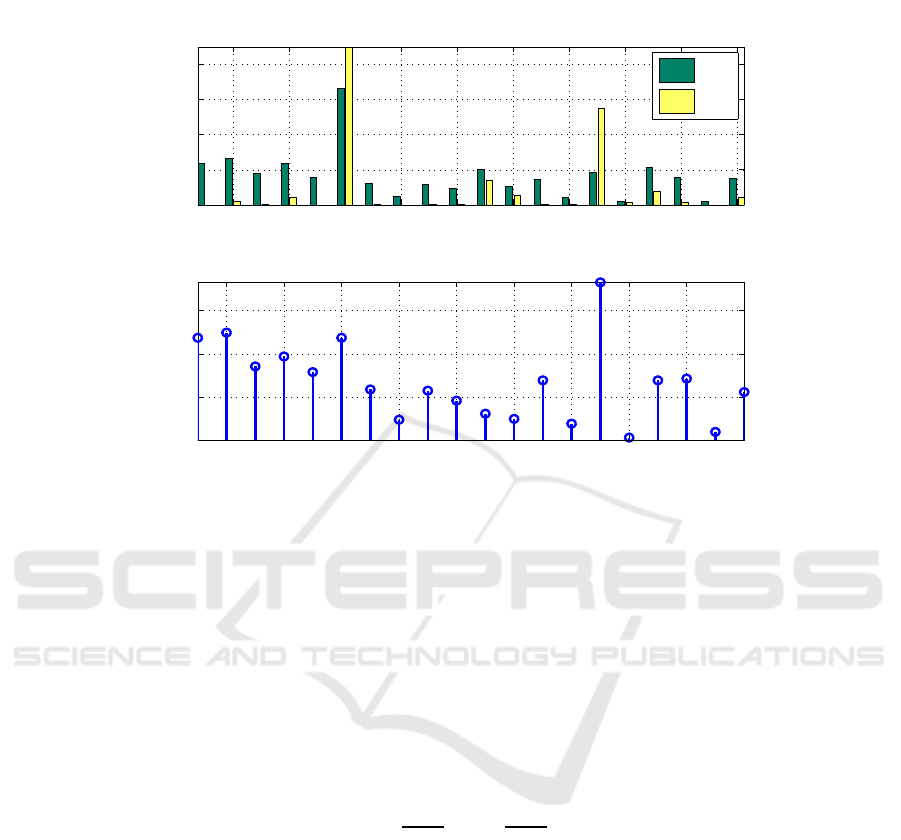
, thus being the considered more relevant. Fig. 1 shows a bar plot of
these quantities, for 20 randomly chosen features of the Example1 dataset, with 2000
training patterns (as described in Subsection 4.1); we also show their ranking value r
i
,
given by (3). For instance, notice that feature 15 is much more informative than feature
6; for feature 6 we have ℓ
(i,−1)
0
= 661 and ℓ
(i,+1)
0
= 998, while for feature 15 these
quantities are ℓ
(i,−1)
0
= 183 and ℓ
(i,+1)
0
= 548. Although, feature 6 has larger ℓ
(i)
0
(thus
it would be considered as more relevant by Method 1), the criterion (3) consideres it as
less informative than feature 15, because it is less asymmetric between classes.
Given a pre-specified maximum number of features m (≤ p), the FS method based
on criterion (3) proceeds as follows.
1. Compute the ℓ
0
norm of each feature, ℓ
(i)
0
, for i ∈ {1, . . . , p}.
2. Remove non-informative features (with ℓ
(i)
0
= 0 or ℓ
(i)
0
= n) on the training set.
If the number of remaining features is less or equal than m, then stop, otherwise
proceed to step 3.
3. Compute the rank r
i
of each feature as defined by (3).
4. Keep only the m features with largest ranks r
i
.
This second method uses class label information, thus being suited only for supervised
classification problems. As in Method 1, we begin by removing the non-informative
always absent (with ℓ
(i)
0
= 0) and always present (with ℓ
(i)
0
= n) features; these features
75

2 4 6 8 10 12 14 16 18 20
0
200
400
600
800
Feature
l
0
(i,−1)
, l
0
(i,+1)
l
0
(i,−1)
l
0
(i,+1)
2 4 6 8 10 12 14 16 18 20
0
100
200
300
Feature
Rank
r
i
Fig.1. The ℓ
(i,−1)
0
and ℓ
(i,+1)
0
values for 20 randomly chosen features of the Example1 dataset
(described in Subsection 4.1), and their rank r
i
= |ℓ
(i,−1)
0
− ℓ
(i,+1)
0
|.
do not contribute to discriminate between classes in the training set. In the case of a
linear SVM, the classifier is defined as a linear combination of the input patterns [17].
The same does not happen with the AdaBoost algorithm, because it depends on the type
of weak classifier(s) that is used.
The criterion (3) was defined for binary problems and in the experiments reported
below we only consider binary problems. There are several possible ways to obtain
related relevance measures for the K-class case, i.e., when c
i
∈ {1, 2, ..., K}. The
natural K-class generalization of the negative entropy criterion (4) is
h
i
=
K
X
k=1
ℓ
(i,k)
0
ℓ
(i)
0
log
2
ℓ
(i,k)
0
ℓ
(i)
0
!
, (5)
with ℓ
(i,k)
0
denoting the ℓ
0
norm of feature i, for class k. A possible generalization of
criterion (3) is
r
i
=
K
X
l=1
K
X
k=1



ℓ
(i,l)
0
− ℓ
(i,k)
0



. (6)
Experiments with these K-class criteria are the topic of future work.
76

4 Experimental Results
In this Section, we present experimental results of the evaluation of our methods. In
Subsection 4.1, we describe the standard BoW datasets used in the experiments; Sub-
section 4.2 describes other feature selection and reduction techniques that we use as
benchmarks. Finally, Subsection 4.3 shows the average test set error rate of SVM and
AdaBoost classifiers on those standard datasets.
4.1 Datasets
The experimental evaluation of the proposed techniques is conducted on the following
three (publicly available) BoW datasets: Spam
1
(where the goal is to classify email
messages as spam or non-spam), Example1
2
, and Dexter
3
(in Example1 and Dexter,
the task is learn to classify Reuters articles as being about “corporate acquisitions” or
not). These datasets have undergone the standard pre-processing (stop-word removal,
stemming) [11]. Table 1 shows the main characteristics of these datasets.
Table 1. The main characteristics of datasets Spam, Example1, and Dexter. The three columns
on the rightmost side show the average values of ℓ
(i)
0
, ℓ
(i,−1)
0
, and ℓ
(i,+1)
0
, for each subset.
Dataset p Subset Patterns +1 -1 ℓ
(i)
0
ℓ
(i,−1)
0
ℓ
(i,−1)
0
Spam 54 — 4601 1813 2788 841.2 411.8 429.4
Example1 9947 Train 2000 1000 1000 9.5 4.5 5.0
Test 600 300 300 2.4 1.1 1.3
Dexter 20000 Train 300 150 150 1.4 0.7 0.7
Test 2000 1000 1000 9.6 – –
Valid. 300 150 150 1.4 0.7 0.7
In the Spam dataset, we have used the first 54 features, which constitute a BoW
representation. We have randomly selected 1000 patterns for training (500 per class)
and 1000 (500 per class) for testing. In the case of Example1, each pattern is a 9947-
dimensional BoW vector. The classifier is trained on a random subset of 1000 patterns
(500 per class) and tested on 600 patterns (300 per class). The Dexter dataset has the
same data as Example1 with 10053 additional distractor features with no predictive
power (independent of the class), at random locations, and was created for the NIPS
2003 feature selection challenge
4
. We train with a random subset of 200 patterns (100
per class) and evaluate on the validation set, since the labels for the test set are not
publicly available; the results on the validation set correlate well with the results on the
test set [8].
We use the implementations of the linear SVM and Modest AdaBoost [18] available
in the ENTOOL
5
toolbox. The weak classifiers used by the Modest AdaBoost G
m
(x)
1
http://archive.ics.uci.edu/ml/datasets/spambase
2
http://kodiak.cs.cornell.edu/svm light/examples/
3
http://archive.ics.uci.edu/ml/datasets/dexter
4
http://www.nipsfsc.ecs.soton.ac.uk
5
http://zti.if.uj.edu.pl/∼merkwirth/entool.htm
77

are tree nodes and we use M =15 (see (1)). The reported results are averages over 10
replications of different training/testing partitions.
4.2 Other Feature Selection/Reduction Methods
To serve as benchmark, we use two other two methods on the TD matrix, and three
different methods on the TDI matrix, as briefly described in this subsection. The first
one is based on the well-known Fisher ratio (FiR) of each feature, which is defined as
FiR
i
=



µ
(−1)
i
− µ
(+1)
i



q
var
(−1)
i
+ var
(+1)
i
, (7)
where µ
(±1)
i
and var
(±1)
i
, are the mean and variance of feature i, for the patterns of each
classes. The FiR measures how well each feature separates the two classes. To perform
feature selection based on the FiR, we simply use the m features with the largest values
of FiR, where m is the desired number of features.
The second method considered is unsupervised being based on random projections
(RP) [1,2, 12] of the TD matrix. Letting A be an m × p matrix, with m ≤ p, we obtain
a reduced/compressed training dataset D
A
= {(y
1
, c
1
), ..., (y
p
, c
p
)}, where
y
i
= Ax
i
, (8)
for i = 1, ..., n. Each new feature in y
i
is a linear combination of the original features in
x
i
. Different techniques and probability mass functions (PMF) have been proposed to
obtain adequate RP matrices [1,2,12]; in this paper, we use the PMF {1/6, 2/3, 1/6}
over {−
p
3/m, 0,
p
3/m}, as proposed in [1].
The third method considered is the (supervised) conditional mutual information
maximization (CMIM) method for binary features [5]. CMIM is a very fast FS tech-
nique based on conditional mutual information; the method picks features that max-
imize the mutual information (MI) with the class label, conditioned on the features
already picked. The mutual information maximization (MIM) method is a simpler ver-
sion of CMIM that uses only the MI between the features and the class label. We apply
these methods on the TDI matrix.
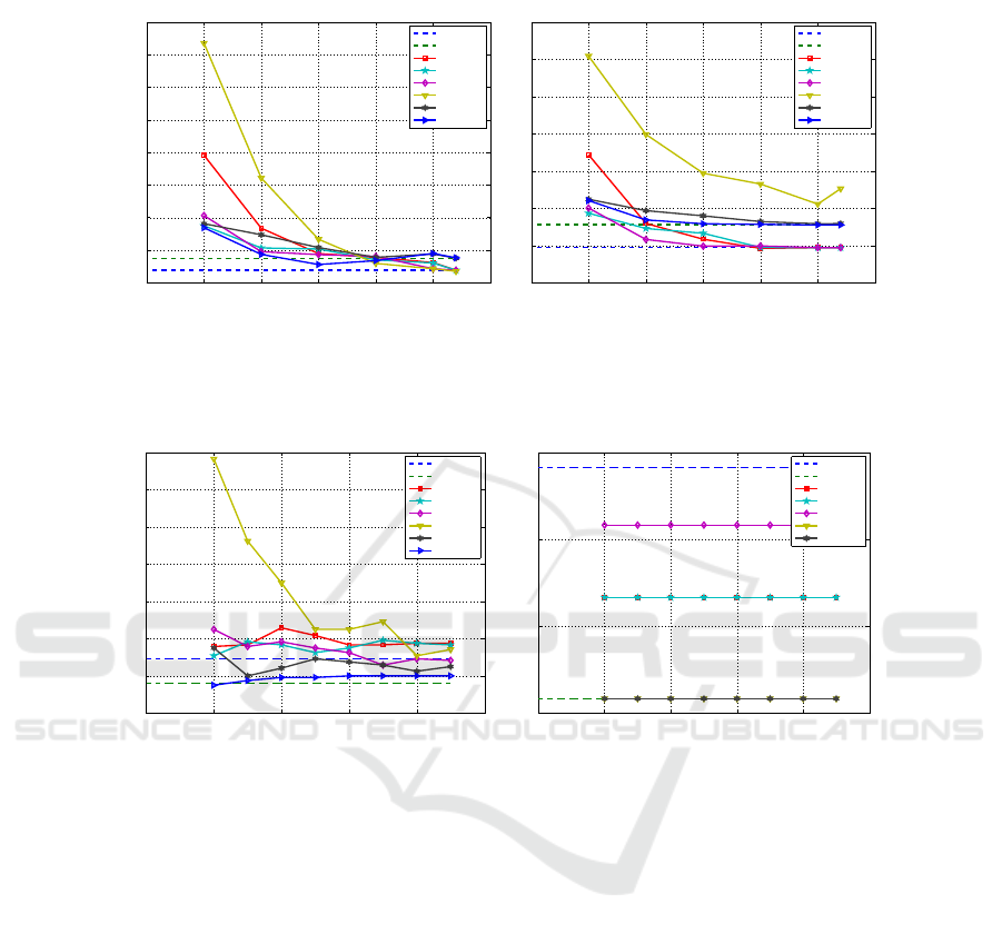
4.3 Test Set Error Rate
Figure 2 displays the test set error rate, as a function of m, for the Spam dataset, using
linear SVM and Modest AdaBoost classifiers based on: the TD matrix, the TDI matrix
with the original number of features; the reduced TD with FS by Method 1, Method
2, FiR, and RP with Achlioptas distribution; the reduced TDI with MIM and CMIM.
Each point is obtained by averaging over 10 replications of the training and test set.
The horizontal dashed lines show the test set error rate for the TD and TDI matrices
without FS or FR. For both classifiers, we have a small difference between the use of
TD and TDI. The SVM classifier obtains a faster descend on the test set error rate than
AdaBoost. The use of RP is not adequate for the AdaBoost classifier. The proposed
78

0 10 20 30 40 50 60
8
10
12
14
16
18
20
22
24
# Features (m)
Test Set Error Rate [%]
Spam with linear SVM
TD
TDI
Method 1
Method 2
Fisher
RP
MIM
CMIM
0 10 20 30 40 50 60
8
10
12
14
16
18
20
22
# Features (m)
Test Set Error Rate [%]
Spam with Modest AdaBoost
TD
TDI
Method 1
Method 2
Fisher
RP
MIM
CMIM
Fig.2. Test Set Error Rate for linear SVM and AdaBoost on Spam dataset (p=54) with 10 ≤ m ≤
54, using TD matrix and its reduced versions by Method 1, Method 2, FI, and RP (Achlioptas
distribution), TDI matrix and its reduced versions by MIM and CMIM.
0 500 1000 1500 2000 2500
4
6
8
10
12
14
16
18
# Features (m)
Test Set Error Rate [%]
Example1 with linear SVM
TD
TDI
Method 1
Method 2
Fisher
RP
MIM
CMIM
0 500 1000 1500 2000 2500
12.5
13
13.5
14
# Features (m)
Test Set Error Rate [%]
Example1 with Modest AdaBoost
TD
TDI
Method 1
Method 2
Fisher
MIM
CMIM
Fig.3. Test Set Error Rate for linear SVM and AdaBoost on Example1 dataset (p=9947) with
500 ≤ m ≤ 2250, using TD matrix and its reduced versions by Method 1, Method 2, FI, and RP
(Achlioptas distribution), TDI matrix and its reduced versions by MIM and CMIM.
Method 2 usually performs better than Method 1, for both classifiers. For m > 30, our
unsupervised Method 1 attains about the same test error rate as the supervised Fisher
ratio. Method 1 also attains better results than RP.
Fig. 3 displays the test set error rate as a function of m, for the Example1 dataset,
with linear SVM and AdaBoost. The proposed methods attain competitive results with
Fishers ratio, being better than RP. With these degrees of reduction, the AdaBoost clas-
sifier is not able to reduce the test set error rate.
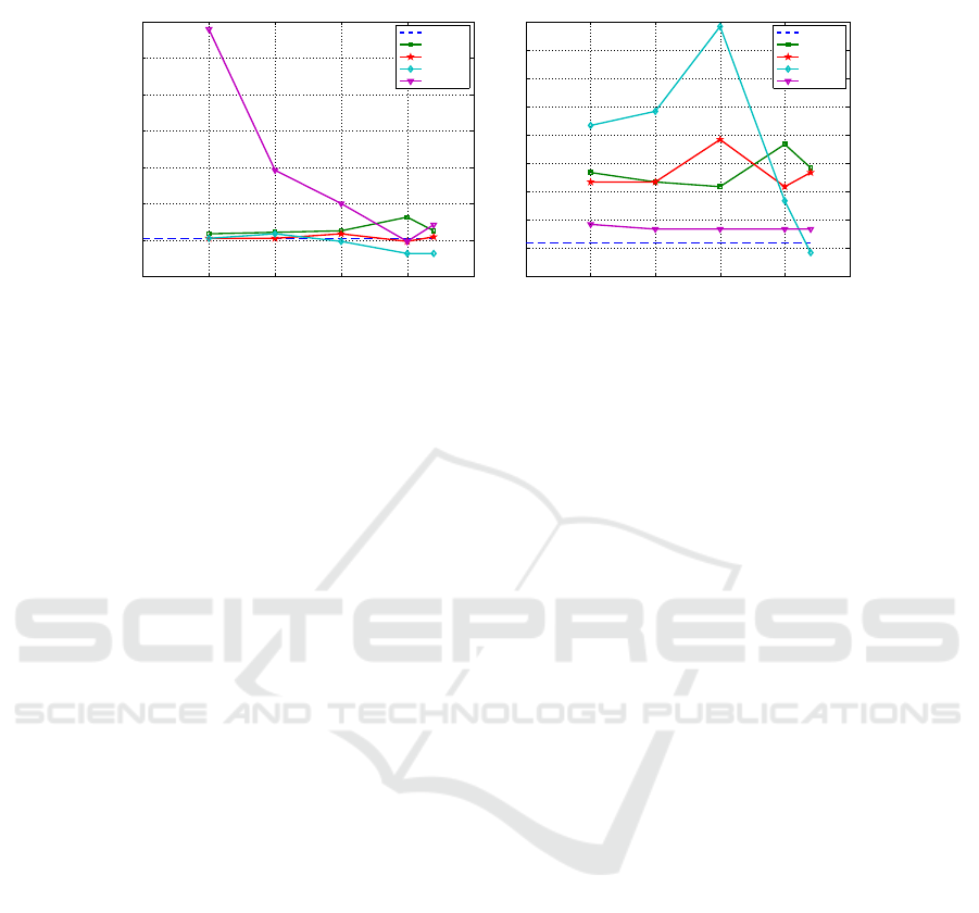
Fig. 4 displays the test results of the linear SVM on the TD and TDI representations
of Dexter dataset. In this case, we apply our methods to both TD and TDI matrices.
On both datasets and both classifiers, the TDI matrix obtains adequate results, as
compared to the TD matrix. On the TD matrix, the RP method is not able to achieve
comparable results to the other techniques, due to the high degree of reduction imposed
on these tests; for larger values of m , we get better results. Our methods obtain similar
79

0 500 1000 1500 2000 2500
6
8
10
12
14
16
18
20
# Features (m)
Validation Set Error Rate [%]
Dexter (TD) with linear SVM
TD
Method 1
Method 2
Fisher
RP
0 500 1000 1500 2000 2500
6
6.5
7
7.5
8
8.5
9
9.5
10
10.5
# Features (m)
Validation Set Error Rate [%]
Dexter (TDI) with linear SVM
TDI
Method 1
Method 2
MIM
CMIM
Fig.4. Validation Set Error Rate for linear SVM on Dexter dataset (p=20000) with 500 ≤ m ≤
2200, using TD matrix and its reduced versions by Method 1, Method 2, FI, and RP (Achlioptas
distribution), TDI matrix and its reduced versions by Method 1, Method 2, MIM, and CMIM.
results to the MIM and CMIM methods on the TDI matrix of Dexter dataset. This
seems to indicate that for this type of data, the information-theoretic FS methods are
not a good choice. The good results of Method 1 on Example1 and Dexter datasets,
leads us to believe that this method can be successfully applied to semi-supervised and
unsupervised problems on sparse high-dimensional datasets.
5 Conclusions
In this paper, we have proposed two methods for feature selection for text classification
problems, using the term-document or the term-document incidence matrices. The first
method works in an unsupervised fashion, without making use of the class label of each
pattern. The second method uses the class label and the ℓ
0
norm to identify the features
with larger significance regarding class separability.
The proposed methods, based on non-zero occurrence counting, have cheaper im-
plementations than the Fisher ratio, random projections, and the information-theoretic
methods based on mutual information. The experimental results have shown that these
methods: significantly reduce the dimension of standard BoW datasets, improving clas-
sification accuracy, with respect to the classifiers trained on the original features; yield
similar results to the Fisher ratio and are better than random projections.
The use of term-document incidence matrices (without reduction) is also adequate,
with both SVM and AdaBoost classifiers. We can thus efficiently represent and classify
large collections of documents with the informationof presence/absenceof a term/word.
Our methods also attained good results on the term-document incidence matrices.
As future work, we will apply Method 1 to semi-supervised learning and we will
modify Method 2 in order to take into account the (in)dependency between features.
We will also explore the use of these methods for multi-class classification problems.
80

References
1. D. Achlioptas. Database-friendly random projections. In ACM Symposium on Principles of
Database Systems, pages 274–281, Santa Barbara, USA, 2001.
2. E. Bingham and H. Mannila. Random projection in dimensionality reduction: applications
to image and text data. In KDD’01: Proc. of the 7th ACM SIGKDD Int. Conf. on Knowledge
Discovery and Data Mining, pages 245–250, San Francisco, USA, 2001.
3. F. Colas, P. Paclk, J. Kok, and P. Brazdil. Does SVM really scale up to large bag of words
feature spaces? In M. Berthold, J. Shawe-Taylor, and N. Lavrac, editors, Proceedings of
the 7th International Symposium on Intelligent Data Analysis (IDA 2007), volume 4723 of
LNCS, pages 296–307. Springer, 2007.
4. F. Escolano, P. Suau, and B. Bonev. Information Theory in Computer Vision and Pattern
Recognition. Springer, 2009.
5. F. Fleuret and I. Guyon. Fast binary feature selection with conditional mutual information.
Journal of Machine Learning Research, 5:1531–1555, 2004.
6. G. Forman. An extensive empirical study of feature selection metrics for text classification.
Journal of Machine Learning Research, 3:1289–1305, 2003.
7. Y. Freund and R. Schapire. Experiments with a new boosting algorithm. In Thirteenth
International Conference on Machine Learning, pages 148–156, Bari, Italy, 1996.
8. I. Guyon, S. Gunn, M. Nikravesh, and L. Zadeh (Editors). Feature Extraction, Foundations
and Applications. Springer, 2006.
9. T. Hastie, R. Tibshirani, and J. Friedman. The Elements of Statistical Learning. Springer,
2nd edition, 2009.
10. K. Hyunsoo, P. Howland, and H. Park. Dimension reduction in text classification with sup-
port vector machines. Journal of Machine Learning Research, 6:37–53, 2005.
11. T. Joachims. Learning to Classify Text Using Support Vector Machines. Kluwer Academic
Publishers, 2001.
12. P. Li, T. Hastie, and K. Church. Very sparse random projections. In KDD ’06: Proc. of the
12th ACM SIGKDD Int. Conf. on Knowledge Discovery and Data Mining, pages 287–296,
Philadelphia, USA, 2006.
13. C. Manning, P. Raghavan, and H. Sch¨utze. Introduction to Information Retrieval. Cambridge
University Press, 2008.
14. E. Mohamed, S. El-Beltagy, and S. El-Gamal. A feature reduction technique for improved
web page clustering. In Innovations in Information Technology, pages 1–5, 2006.
15. R. Schapire and Y. Singer. Boostexter: A boosting-based system for text categorization.
Machine Learning, 39((2/3)):135–168, 2000.
16. K. Torkkola. Discriminative features for text document classification. Pattern Analysis and
Applications, 6(4):301–308, 2003.
17. V. Vapnik. The Nature of Statistical Learning Theory. Springer-Verlag, 1999.
18. A. Vezhnevets and V. Vezhnevets. Modest adaboost - teaching adaboost to generalize better.
Graphicon, 12(5):987–997, September 2005.
81