
VEHICLE ROUTING TO MINIMIZE MIXED-FLEET FUEL
CONSUMPTION AND ENVIRONMENTAL IMPACT
O. Gusikhin
1
, P. MacNeille
1
and A. Cohn
2
1
Ford Motor Company Research and Innovation Center, 2101 Village Road, Dearborn, MI 48121, U.S.A.
2
University of Michigan, 2797 IOE Building, 1205 Beal Avenue, Ann Arbor, MI 48019, U.S.A.
Keywords: Fuel Economy, Heterogeneous Vehicle Routing Problem, Optimization.
Abstract: Efficient vehicle routing is critical to the operational profitability and customer satisfaction of vehicle fleet-
related businesses, especially in light of increasing, and highly volatile, fuel prices. Growing pressures to
reduce negative environmental impacts have suggested that a second metric (vehicle emissions) should also
be considered in vehicle routing. Currently, the majority of existing tools use distance as a surrogate for
cost. When considering a mixed fleet of multiple vehicle types, with individual vehicles within a fleet type
also varying by age and vehicle health, this surrogate becomes significantly less accurate. Furthermore,
using distance as a surrogate fails to capture the variations between city and highway driving, which are
particularly striking for hybrid vehicles. We thus propose a new approach to the vehicle routing problem,
specifically targeting applications with mixed fleets including clean-vehicle technologies, in recognition of
the limitations of the existing approaches.
1 INTRODUCTION
Efficient vehicle routing is critical to the operational
profitability and customer satisfaction of vehicle
fleet-related businesses. The rising and highly-
variable cost of fuel, as highlighted by the price
spike in the summer of 2008, increases the
importance of efficient vehicle routing. At the same
time, growing environmental concerns suggest that
cost is not the only metric of importance and that
emissions should also be taken into account.
Currently, the majority of existing methods and
software packages minimize travel distance as a
surrogate for cost. Although there is a positive
correlation between distance traveled and fuel
consumed, it is not a perfect correlation. In
particular, both fuel efficiency and emissions vary
depending upon driving conditions (e.g. city vs.
highway driving). This variability is even more
pronounced in a heterogeneous fleet comprised of
multiple vehicle types with a range of fuel-
consumption and emissions characteristics.
In recent years, socio-economical pressures to
reduce their fuel costs and carbon dioxide (CO
2
)
footprint have motivated many fleet operators to
begin upgrading their fleets, focusing on clean-
vehicle technologies and alternative fuels, including
flex-fuel, hybrid vehicles, and plug-in hybrid electric
vehicles (PHEV). As a result, many commercial
fleets are currently composed of a heterogeneous set
of vehicles, with noticeable variations in fuel
economy and emissions across vehicle type.
Furthermore, there are variations across vehicles
even within a given vehicle type or common set of
capabilities, because newer vehicles typically exhibit
better fuel economy and better emission control
technologies than older vehicles.
Consider the following examples of highly
heterogeneous fleets: Florida Power and Lighting
(www.fpl.com), the leader in green fleet initiatives,
has a fleet of approximately 2400 vehicles, with half
of the fleet powered by biodiesel, 300 hybrids and
plug-in hybrids now in service, and plans to convert
one-third of the vehicles to hybrid by the end of
2010.
A key issue in incorporating the fuel efficiencies
and emissions of heterogeneous fleets within the
vehicle routing problem is this: The differences in
fuel efficiencies and emissions across vehicle types
are not exclusively proportional to the distance
traveled, but are also highly dependant on the
driving cycle. For instance, a hybrid vehicle takes
advantage of the regenerative braking that occurs in
stop-and-go driving environments to charge a
battery which can then be used to power the vehicle
285
Gusikhin O., MacNeille P. and Cohn A. (2010).
VEHICLE ROUTING TO MINIMIZE MIXED-FLEET FUEL CONSUMPTION AND ENVIRONMENTAL IMPACT.
In Proceedings of the 7th International Conference on Informatics in Control, Automation and Robotics, pages 285-291
Copyright
c
SciTePress

when traveling at slow speeds. On average, fuel
consumption is reduced about 20% by regenerative
braking (Chan and Chau, 2001). Conversely, in
highway driving, hybrids provide minimal, if any,
improvement in fuel efficiencies over their
conventional counterparts.
The introduction of PHEVs, which use
electrically-charged batteries for the initial portion
of a trip and revert to gasoline-based power only
when the battery has been depleted, presents even
greater variability in terms of the correlations
between distance and fuel utilization.
When we move beyond fuel costs to also
consider the environmental impact of vehicle
routing, the complexity grows further. Fuel
consumption is effectively proportional to CO
2
emission, so fuel economy improvements are
reflected in CO
2
reduction. Additionally, there may
be requirements to minimize or eliminate
conventional emissions such as volatile organic
components (VOC) and nitrogen oxides (NO
x
)
emissions in highly populated areas, requiring the
use of electric power or other clean alternative fuel
options and thus limiting the feasible region of a
vehicle routing problem.
In this paper, we consider ways to explicitly
capture fuel consumption and emissions in a mixed-
fleet vehicle routing program and analyze the
opportunities for simultaneously reducing costs and
negative environmental impacts. In Section 2, we
review factors that influence fuel consumption and
emissions and consider ways to estimate these
metrics for a given route. In Section 3, we suggest a
number of formulations for this new variation of the
vehicle routing problem. We also outline a solution
approach based on composite variable modeling. In
Section 4, we provide a numerical example and
analysis to highlight the benefits of our proposed
approach and we then offer conclusions and
suggested areas for future research in Section 5.
2 ESTIMATION OF FUEL
ECONOMY & VEHICLE
ENVIRONMENTAL IMPACT
Route planning is done by representing the road
system as a graph in which intersections are nodes
and road segments are arcs. To determine the best
route from an origin node to a destination node, each
arc is associated with a cost that represents distance,
travel time, or fuel consumption. Then Dijkstra's
algorithm (or an equivalent) is used to find the
lowest cost path which is then inversed mapped to
the road system for visualization and navigation of
the preferred route.
Total fuel cost along a given route is the product
of the total consumption of each type of fuel and the
per-unit cost for that fuel. Total fuel consumption
along an arc is largely dependant on the vehicle
specific load (VSL) opposing vehicle motion
multiplied by the distance traveled against the VSL
to give the total energy required to travel the arc.
This energy can be readily converted into fuel. For
example, about 0.003 gallons of gasoline or 0.002
kWh of electricity are needed to push against a
pound of force over a one mile stretch of road. These
factors will vary, however; with the efficiency of the
energy conversion which depends on many factors.
The VSL depends largely on external factors that
include the drive cycle, aerodynamic drag, rolling
resistance, parasitic drag, and gradient drag. These
factors in turn are dependant on several external
factors including weather conditions, road and traffic
conditions and topography. Most of the external
factors can be reasonably well estimated using well
known engineering formulas; however, the VSL also
depends on the pattern of acceleration/deceleration
that takes place along the branch. Driving pattern
effects depend largely on complex interactions
between the driver, the road, the powertrain, and
traffic conditions. Thus, these effects are difficult to
predict.
One approach to predicting these complex
factors is by classifying road, traffic, and driver and
drivetrain combinations into load effects. The US
Environment Protection Agency (EPA) provides
miles per gallon estimates for highway and city for
all vehicles sold in the US in the last 15 years
currently based on two standard driving cycles.
Although these estimates may not be adequate to
accurately forecast the specific fuel consumption,
they nevertheless can provide a reasonable basis for
the comparative analysis between different vehicles.
A more detailed classification is described in
Brundell-Freij and Ericsson (Brundell-Freij and
Ericsson, 2005), where a classification system has
been developed based on extensive data collected
from instrumented vehicles. Four variables relating
to the road type were found to be significant: 1)
occurrence and density of junctions controlled by
traffic lights, 2) speed limit, 3) function of the street,
and 4) the type of neighborhood. A large effect was
attributed to the power-weight ratio of the vehicle,
which presumably is descriptive of the drivers that
choose a vehicle with a specific power-weight ratio.
ICINCO 2010 - 7th International Conference on Informatics in Control, Automation and Robotics
286

A challenge in using instrumented vehicles is in the
ability to collect adequate data. For example, in the
Brundell-Freij and Ericsson study much of the data
was collected in Lund, Sweden. This location has
limited topography, so road gradient was not
captured, although it is well known that road
gradient is an important factor in situations with
topographic relief. For example, (Tavares et al.,
2009) develops a topography-based routing
algorithm for waste collection vehicles in a
mountainous area and demonstrates that the
proposed approach allows reduction of fuel
consumption despite increasing in the distance
traveled. Also road design and traffic control
policies may vary considerably between political
jurisdictions, as may the mix of vehicles. One way to
overcome these difficulties is to use vehicle and
traffic modeling to determine the significant factors
for classification.
Modeling tools such as the Powertrain System
Analysis Toolkit (PSAT) (PSAT, 2008) or The
MathWorks Simulink/SimDriveLine (Rose-Hulman,
2005) can be used to estimate the energy or fuel
along a route given vehicle design parameters,
external load factors such as road gradient and the
driver's torque demand along the route. Vehicle
design parameters can be obtained from vehicle
manufacturers and external factors from published
maps. Driver's torque demand involves the
psychophysics of driving and has been simulated
using software such as VISSIM
or MISSION (PTV
AG, 2009), (Wiedemannn et al., 1991), (Busawon et
al., 2006), (Noland and Quddus, 2006).
Vehicles in the fleet may be instrumented to
collect actual fuel economy data along the branches
they travel. The data may be recovered from the
vehicle at a download site and stored in a database.
Periodically the database may be used to
automatically refine the costs assigned to a class of
road segments, and to reclassify segments as needed.
3 VEHICLE ROUTING TO
MINIMIZE FUEL
CONSUMPTION
The Vehicle Routing Problem to Minimize Mixed-
Fleet Fuel Consumption and Environmental Impact
(VRPMF) belongs to the class of heterogeneous fleet
vehicle routing problems (HVRP). (Baldacci et al.,
2008) provides a comprehensive classification and
review of the main approaches proposed for VRP
with a heterogeneous fleet. Specifically, the problem
being considered in the paper represents a variant of
HVRP with Vehicle-Dependent Routing Costs
(HVRPD). They note that solution approaches to
this difficult family of problems, both in the
literature and in commercial applications, have
predominantly been heuristic in nature. These are
typically adaptations or extensions of solution
techniques for traditional VRP and VRP with Time
Windows.
In order to capture the complexities (and, in
particular, the non-linearities) of VRPMF, we
instead propose to leverage the use of composite
variable modeling (CVM) to capture the complex
real-world details associated with accurately
modeling the fuel cost (and associated emissions) of
a prescribed route. The idea behind CVM (Cohn,
2002), (Barlatt, et al., 2009) is to embed modeling
complexity into the variable definition rather than
capturing it explicitly in a model which may then
become intractable. For example, in VRPMF,
explicitly modeling the cost functions described in
Section 2 within the framework of a traditional VRP
would make an already difficult problem unsolvable.
However, it is far easier to calculate the cost of a
given route (for a given vehicle) off-line. We can
then formulate a master problem in which each
variable represents the assignment of a specific route
to a specific vehicle. For a given route, we can
compute the total fuel consumption for a given
vehicle, and thus the total cost is just the sum of the
chosen assignments. Similarly, a route pre-specifies
all the customer demands that it meets, and thus we
only need two sets of constraints. The first ensures
that each vehicle is assigned to at most route and the
second ensures that each customer demand is met
exactly once.
The challenge, then, is to address the
exponentially large number of potential variables.
Clearly not all of the exponentially-large set of
feasible routes (and their corresponding costs) can
be generated. Even if they could, it would not be
possible to solve the resulting exponentially-large
set partitioning problem. Instead, column generation
techniques (Desaulniers et al., 2005) (originally
developed as part of Dantzig-Wolfe Decomposition)
can be employed. The idea behind column
generation for solving a linear program with an
exponential number of variables is to identify
candidate pivot variables for the simplex method not
by pricing each variable’s reduced cost directly, but
rather by solving a secondary optimization problem
(often called a sub problem) which seeks the feasible
variable with the most negative reduced cost. If this
yields a negative reduced cost variable, then the
VEHICLE ROUTING TO MINIMIZE MIXED-FLEET FUEL CONSUMPTION AND ENVIRONMENTAL IMPACT
287

simplex pivot occurs and the algorithm proceeds. If
the most negative reduced cost variable is strictly
non-negative, then a certificate of optimality is
achieved and the algorithm terminates with a
provably-optimal solution.
In Dantzig-Wolfe Decomposition, the inherent
structure of a problem leads to a sub-problem that is
pre-defined. Furthermore, it is itself a linear program
and thus straightforward to solve. In CVM, because
the variable definition is chosen specifically to
overcome challenges of a traditional formulation, the
sub problem reflects these challenges.
Perhaps the most closely related work to our
proposed approach is that of Taillard (Taillard,
2005), who used a heuristic based on column
generation techniques to solve HVRPD.
Specifically, a large set of candidate routes were
generated by solving separate homogeneous VRP
problems for each fleet type. The final routes were
then selected using a set partitioning formulation to
ensure that all demands were met.
A key difference between our proposed approach
and typical network-based routing problems is that
the “cost” of a route cannot be computed simply by
adding the individual arc costs (if so, the sub-
problem would be a simple minimum cost flow
problem). At first glance, it seems possible to
formulate the sub problem as a network flow
problem, where each node represents a customer or
depot, each arc represents the driving from one node
to another, and the cost associated with each arc can
fully capture (based on off-line calculations) the cost
of this driving. This is not quite true, however: The
cost on a given arc is not independent of the other
arcs that are also chosen for an individual vehicle’s
route. This is because the fuel consumption on an
arc depends on the starting conditions of the vehicle
at the first node. If the battery is fully charged, it
may be possible to complete most of the driving
without relying on gasoline, and the resulting cost
will be lower, whereas if the battery is depleted, the
cost of the arc will be much higher.
Therefore, a more sophisticated approach to
solving the sub-problem must be employed. For
example, we could take a multi-label shortest path
approach (Desrochers and Soumis, 1988), which is
similar to Dijkstra’s shortest path algorithm, but
with an added layer of complexity. Specifically,
multiple metrics (not just cost) must be checked to
determine whether a partial path can be pruned from
consideration. One partial path dominates another
only if it is less costly and covers the same amount
of demand or more and has the same amount of
remaining battery charge or more. Efficiently
solving this sub-problem is the key to successfully
solving the master problem.
We conclude this section by noting that this
approach has the added advantage of allowing the
user to trade off between time and solution quality.
Specifically, the solution quality continues to
improve as each new candidate route is added to the
master problem for consideration, but high-quality
feasible solutions can nonetheless often be found
early in the process. Furthermore, this approach
naturally lends itself to a parallel implementation. At
the highest level, a separate sub-problem can be
solved, in parallel, for each vehicle. Furthermore,
these individual sub-problems themselves can
leverage a parallel architecture for efficient search.
4 ILLUSTRATIVE EXAMPLE
This section provides a simplified illustrative
example of VRPMF. We consider a fleet of two
vehicles: the first is a 2009 Ford Taurus front-wheel
drive gasoline engine vehicle and the second is 2010
Ford Escape 4-wheel drive hybrid vehicle. Figure 1
shows estimates of the miles per gallon (MPG)
values and environmental scores as provided by the
US Environmental Protection Agency (EPA) at
www.fueleconomy.gov. Note that the Taurus gets 18
MPG in city driving and 28 MPG in highway
driving, while the Escape hybrid gets 27 MPG on
the highway and 30 MPG in the city. The
environmental impact of each vehicle can be
evaluated by its carbon footprint and air pollution
score. The carbon footprint measures greenhouse gas
emissions (primarily CO
2
) that in turn impact
climate change. CO
2
emissions are closely linked to
fuel consumption, since CO
2
is the ultimate end
product of burning gasoline. The Air Pollution score
represents the amount of health-damaging and
smog-forming airborne pollutants (such as carbon
monoxide, CO, and oxides of nitrogen, NOx) that
the vehicle emits on a scale from 0 (worst) to 10
(best). Note that there is little correlation between
fuel consumption and these emissions; emissions
primarily depend on the emission control
technology. Taurus has an Air Pollution score of 6
and Escape Hybrid has a score of 8.
Suppose that we have eight customers distributed
within a given geographical area as shown in Figure
2. The customers are labeled 1 to 8, while 0 is the
depot. The driving distance between the depot and
each of the customer sites is presented in Table 1.
For this example, we assume that the distance data is
symmetrical and shown as X+Y, where X is the
ICINCO 2010 - 7th International Conference on Informatics in Control, Automation and Robotics
288
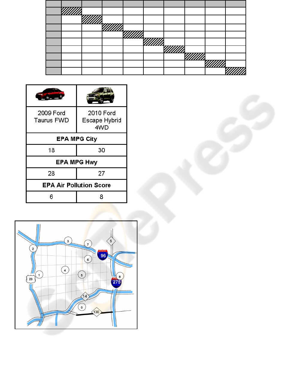
Table 1: Distance between depot and between customer's sites.
012 3456 78
0
14.5+ .9 19+ 1 23.9+ 2.4 0+ 11.6 0+ 9.8 0+ 13.6 12.5+ 10 15.5+ 1.1
1
14.5+ .9 4.2+ 1.5 10.2+ 1.8 0+ 6.3 0+ 10.3 0+ 12.1 12.2+ 2.6 0+ 17.9
2
19+ 1 4.2+ 1.5 5.7+ 2.2 2.5+ 9.1 4.2+ 11.6 11.4+ 4.7 7.7+ 2.9 20.2+ 2
3
23.9+ 2.4 10.2+ 1.8 5.7+ 2.2 0+ 6.7 0+ 10.6 0+ 6.5 0+ 3.8 14.3+ 1.5
4
0+ 11.6 0+ 6.3 2.5+ 9.1 0+ 6.7 0+ 4 14+ 6 17+ 7.5 0+ 11.6
5
0+ 9.8 0+ 10.3 4.2+ 11.6 0+ 10.6 0+ 4 0+ 3.8 0+ 8.6 0+ 7.7
6
0+ 13.6 0+ 12.1 11.4+ 4.7 0+ 6.5 14+ 6 0+ 3.8 0+ 4.7 7.4+ 4.1
7
12.5+ 10 12.2+ 2.6 7.7+ 2.9 0+ 3.8 17+ 7.5 0+ 8.6 0+ 4.7 12.5+ 2.5
8
15.5+ 1.1 0+ 17.9 20.2+ 2 14.3+ 1.5 0+ 11.6 0+ 7.7 7.4+ 4.1 12.5+ 2.5
Figure 1: Fleet Composition.
Figure 2: Vehicle Routing Problem.
number of highway miles and Y is the number of
city miles.
Further, we assume that each service call
requiresapproximately 90 minutes and that each
service agent has to finish his/her route, starting and
ending at the depot, within 8 hours.
We ignore breaks, and assume that there is no
capacity limit on the routes other than the time limit.
We begin by solving the traditional problem of
minimizing the total fleet vehicle miles traveled
(VMT). (In this small problem, this can be done by
explicit enumeration). The total optimum VMT is
97.2. One vehicle visits customers 1, 2, 3, and 4 with
a total travel distance of 47.3 miles, comprised of
22.9 city miles and 24.4 highway miles. The other
vehicle visits customers 5, 6, 7, and 8 with a total
travel distance of 49.9 miles, comprised of 21.9 city
miles and 28 highway miles. The estimated travel
time for the first route is 75 minutes and for the
second route is 78 minutes. Note that in this
variation of the problem, we do not differentiate
between vehicles, as we are simply minimizing
distance traveled.
For illustrative purposes, to estimate fuel
consumption of each vehicle along the given routes
we assume the estimated highway and city MPGs as
defined in Figure 1. (Of course, real-world
calculations are more complex as we discussed in
section 2). As a result, the fuel consumption of the
Taurus for the first route is 2.14 gallons and for the
second route is 2.22 gallons. For the Escape Hybrid,
the first route consumes 1.67 gallons and the second
route consumes 1.77 gallons.
The optimal solution is to assign the Taurus to
the first route, resulting in the consumption of 2.14
gallons, and to assign the Escape to the second route,
with an estimated consumption of 1.67 gallons of
gasoline. The total fleet fuel consumption for the
given solution is 3.81 gallons of gasoline. The
results are presented graphically in Figures 3 and 4.
VEHICLE ROUTING TO MINIMIZE MIXED-FLEET FUEL CONSUMPTION AND ENVIRONMENTAL IMPACT
289
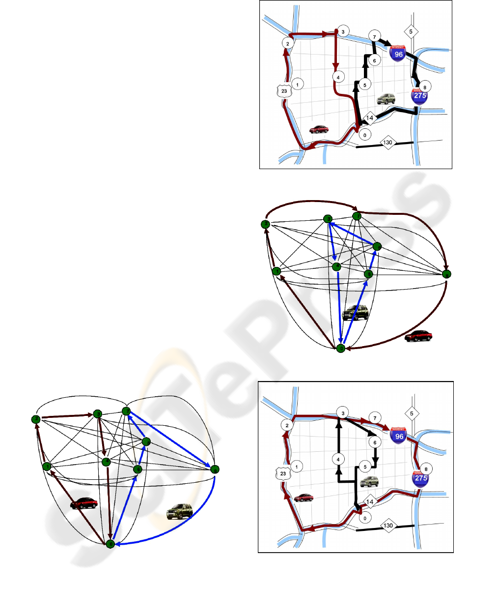
We next reformulate the problem to take into
account fuel economy, i.e. distinguishing in our
optimization between highway and city driving, and
treating the two vehicles separately, in recognition
of their distinct characteristics. The optimal solution
for this problem is presented in Figures 5 and 6.
Although the VMT increases (from 97.2 to
101.7), the fuel consumption decreases from 3.81 to
3.72 gallons. Note that the optimal routes have
changed (see Figure 4). The route served by the
Taurus covers customers 1, 2, 7, and 8 with a total
length of 63.3 miles, but of this 54.4 miles is
highway driving and only 8.9 miles is city driving.
Conversely, the Escape Hybrid is assigned to a route
that serves customers 5, 6, 3, and 4, using only city
driving (for a total length of 38.4 miles).
Table 2 provides a comparative summary of the
two solutions. In addition to the economical impact,
this demonstrates how a reduction in fuel
consumption also leads to a reduction in
environmental impact from the fleet operations. First
of all, the reduction of fuel consumption reduces the
CO
2
emissions. In addition, the second solution
shifts the time the Taurus spends in the city routes to
the Escape Hybrid. As is shown in Figure 1, the
Taurus has a lower EPA Air Pollution Score than the
Escape Hybrid. Consequently the second solution
also reduces health-damaging and smog-forming
airborne pollutants along populated areas. We could
also capture this explicitly in the objective function
of our formulation, either by specifying constraints
on the total Air Pollution Score (possibly weighted
by the location of the route arcs), or by introducing
weights in the objective function.
Figure 3: Solution 1 Graph.
Figure 4: Solution 1 Map.
Figure 5: Solution 2 Graph.
Figure 6: Solution 2 Map.
ICINCO 2010 - 7th International Conference on Informatics in Control, Automation and Robotics
290

Table 2: Comparative summary of two VRT solutions.
5 CONCLUSIONS
In this paper we discuss the importance of the
heterogeneous fleet vehicle routing problem based
on fuel consumption rather than just distance
traveled. We describe the complex function that
determines how much fuel a given route consumes,
and argue that distance is an inadequate surrogate
when multiple fleet types, especially varying across
different technologies, are used. We provide a
simple example to illustrate how minimizing total
miles traveled can yield a very different solution
than minimizing fuel consumption. We also discuss
solution techniques, specifically based on the use of
composite variable modeling, to solve this
computationally challenging problem.
In the future, we propose to consider emissions
as well as explicit fuel costs (which implicitly
capture CO
2
emissions but not NO
x
). We also
suggest extending VRPMF to include variations and
extensions such as those studied in the basic VRP,
such as balancing routes, satisfying time windows,
etc.
REFERENCES
Chan, C. C. and Chau, K.T.; Modern Electric Vehicle
Technology. Oxford University Press Nov. 15, 2001.
Brundell-Freij, K. and Ericsson, E.; Influence of street
characteristics, driver category and car performance on
urban driving patterns, Transportation Research Part D
10, 2005, pp. 213-229.
Tavares, G., Zsigraiova, Z., Semiao, V., Carvalho, M.G ,
Optimization of MSW collection routes for minimum
fuel consumption using 3D GIS modeling, Waste
Management 29, 2009, pp. 1176–1185.
PSAT Overview, January 2008, http://
www.transportation.anl.gov/pdfs/HV/412.pdf
Rose-Hulman Institute of Technology; Rose-Hulman
Institute of Technology Students Design Hybrid
Vehicle Powertrain with Simulink and SimDriveLine,
2005; http:// www.rose-hulman.edu/ challengex/
downloads/Rose-Hulman_user_story.pdf
PTV AG, VISSIM – State-of-the-Art Multi-Modal
Simulation; http:// www. ptvag. com/ fileadmin /
files_ptvag.com/download/traffic/Broschures_Flyer/V
ISSIM/VISSIM_Brochure_e_2009_HiRes.pdf, 2009.
R. Wiedemann, U. Reiter, Wiedemann Model-
Microscopic Traffic Simulation The Simulation
System Mission, 1991; http://
www.ptvamerica.com/fileadmin/files_ptvamerica.com
/library/1970s%20Wiedemann%20VISSIM%20car%2
0following.pdf
Roshan Busawon, M. David Checkel, CALMOB6: A Fuel
Economy and Emissions Tool for Transportation
Planners, presented to the Best Practices in Urban
Transportation Planning session of the 2006 Annual
Conference of the Transportation Association of
Canada, Charlettetown, Price Edward Island, 2006.
Robert B. Noland, Mohammed A. Quddus, Flow
improvements and vehicle emissions: Effects of trip
generation and emission control technology,
Transportation Research Part D 11, 2006, pp. 1-14.
Roberto Baldacci, Maria Battarra, and Daniele Vigo,
Routing a Heterogeneous Fleet of Vehicles in
B. Golden, et al. (Eds), The Vehicle Routing Problem:
Latest Advances and New Challenges, Springer 2008,
pp. 3-27.
Cohn, A. “Composite Variable Modeling for Large-Scale
Problems in Transportation and Logistics,” doctoral
dissertation in Operations Research, Massachusetts
Institute of Technology, advised by Dr. Cynthia
Barnhart, April 2002.
Barlatt A.,Cohn A.,FradkinY., Gusikhin O.; Morford C.,
Using composite variable modeling to achieve realism
and tractability in production planning: An example
from automotive stamping, IIE Transactions, Volume
41, Issue 5, 2009 , pp. 421 – 436.
Desaulniers, G., J. Desrosiers, and M. Solomon, editors.
“A Primer in Column Generation.” Springer US, 2005.
Taillard E. D., A heuristic column generation method for
the heterogeneous VRP, Operations Research --
Recherche opérationnelle 33 (1), 1999, pp. 1-14.
(Publication CRT-96-03, Centre de recherche sur les
transports, Université de Montréal, 1996. Revision
11.2005)
Desrochers, M. and F. Soumis. A Generalization
Generalized Permanent Labeling Algorithm for the
Shortest Path Problem with Time Windows. INFOR
1988 26:191 – 212.
VEHICLE ROUTING TO MINIMIZE MIXED-FLEET FUEL CONSUMPTION AND ENVIRONMENTAL IMPACT
291
