EFFICIENT 3D DATA COMPRESSION THROUGH

PARAMETERIZATION OF FREE-FORM SURFACE PATCHES

Marcos A. Rodrigues, Alan Robinson and A. Osman

Geometric Modelling and Pattern Recognition Research Group, Shefﬁeld Hallam University, Shefﬁeld, U.K.

Keywords:

3D data compression, Surface parameterization, 3D reconstruction.

Abstract:

This paper presents a new method for 3D data compression based on parameterization of surface patches.

The technique is applied to data that can be deﬁned as single valued functions; this is the case for 3D patches

obtained using standard 3D scanners. The method deﬁnes a number of mesh cutting planes and the intersection

of planes on the mesh deﬁnes a set of sampling points. These points contain an explicit structure that allows us

to deﬁne parametrically both x and y coordinates. The z values are interpolated using high degree polynomials

and results show that compressions over 99% are achieved while preserving the quality of the mesh.

1 INTRODUCTION

Cheap storage and secure transmission of 3D data

bring advantages to a number of applications in se-

curity, engineering, CAD/CAM collaborative design,

medical visualization, entertainment and e-commerce

among others. We have developed and demonstrated

original methods and algorithms for fast 3D scanning

for a number of applications with particular focus on

security (Robinson, 2004), (Brink, 2008), (Rodrigues,

2008), (Rodrigues, 2009). Our algorithms can per-

form 3D reconstruction in 40ms and recognition in

near real-time, in just over one second per subject.

This paper is concerned with compression of 3D

data for fast transmission over the Internet. A re-

alistic scenario we are exploring involves 3D facial

biometric veriﬁcation at airports. The method is

non-intrusive and aims at minimal disruption and is

based on our past experience with 3D biometrics at

Heathrow Airport (London, UK) in 2005. An enroll-

ment shot is taken and reconstructed in 3D at an au-

tomated check-in desk, where a new database is cre-

ated for each ﬂight. At the gate, before boarding the

plane another 3D shot is taken for veriﬁcation. The

created databases are transmitted to the local Police

who would perform a search against their records. If

the Police ﬁnd no information to warrant keeping the

data for longer, all data must be erased after a time

lapse, normally within 24 hours. For international

ﬂights and where no mechanisms for sharing infor-

mation between Police Forces are available, the data

can be transmitted to the destination Police authorities

before the ﬂight actually arrives at the destination.

A signiﬁcant constraint of this scenario is that 3D

ﬁles are very large; a high deﬁnition 3D model of a

person’s face is around 20MB. For a ﬂight with 400

passengers, this would mean to dispatch 8GB of data.

If we consider the number of daily ﬂights in a medium

sized airport, we soon conclude that this may be un-

workable. It is clear that methods to compress 3D data

would be beneﬁcial to the scenario considered here

but, more importantly, would represent an enabling

technology for a potential large number of other ap-

plications.

Although some standards exist for 3D compres-

sion such as Java 3D and MPEG4, the compression

rates are still low for general sharing of ﬁles over the

Internet. In general there are three methods one can

use to share 3D data. The ﬁrst method is based on im-

age compression where each snapshot of a 3D scene

is compressed as a 2D image. The second method is

based on hierarchical reﬁnement of a 3D structure for

transmission, where a coarse mesh is followed by in-

creasing reﬁnements until the original, full 3D model

is reconstructed at the other end. The third method

is based on mesh compression where algorithms tra-

verse the mesh for local compression of polygonal re-

lationships.

Compression methods are focused on represent-

ing the connectivity of the vertices in the triangu-

lated mesh. Examples include the Edgebreaker al-

gorithm (Szymczak, 2000) and (Szymczak, 2002).

Products also exist in the market that claim a 95%

lossless ﬁle reduction such as from 3D Compression

130

Rodrigues M., Robinson A. and Osman A. (2010).

EFFICIENT 3D DATA COMPRESSION THROUGH PARAMETERIZATION OF FREE-FORM SURFACE PATCHES.

In Proceedings of the International Conference on Signal Processing and Multimedia Applications, pages 130-135

 SciTePress

Technologies Inc (3DCT, 2010) for regular geomet-

ric shapes. Other techniques for triangulated models

include the work of (Shikhare, 2002) and vector quan-

tization based methods (Hollinger, 2010) where rates

of over 80:1 have been achieved.

The 3D compression method proposed in this pa-

per was devised from our research on fast 3D acquisi-

tion using light structured methods (Robinson, 2004),

(Rodrigues, 2008), (Brink, 2008), (Rodrigues, 2009).

The 3D scanning method is based on splitting the pro-

jection pattern into light planes. Each plane hits the

target object as a straight line and the apparent bend-

ing of the light due to the position of the camera in

relation to the projection allows us to calculate the

depth of any point along the projected light plane.

Taking full advantage of such properties, our method

is closer to polygonal mesh compression but with sig-

niﬁcant differences as it does not depend on search-

ing for local relationships that are most susceptible to

compression. We have achieved compression rates of

free-form surface patches that drastically reduce the

original 3D data by over 99% to a plain text ﬁle. Once

in plain text, it can be encrypted and securely trans-

mitted over the network and reconstructed at the other

end.

This paper is organized as follows. Section 2

presents the method and Section 3 describes the in-

stantiation of the method to surface patches. The data

are compressed and reconstructed and a comparative

analysis of polynomials of various degrees is pro-

vided. Finally a conclusion is presented in Section 4.

2 METHOD

2.1 The Surface Patch as an Explicit

Function of Two Variables

The method presented here applies to surface patches

acquired by standard 3D scanning techniques. Any

such patch can be described as a single valued shape

in one dimension where their values are represented

as an explicit function of two independent variables.

The height of a point is represented by their z-value

and we can say that the height of a function (x, y)

is some function f (x,y). The advantage of a single-

valued function is that it has a simple parametric form,

P(u,v) = (u,v, f (u,v)) (1)

with normal vector n(u, v) = (−δ f /δu, −δ f /δv, 1).

Both u and v are the dependent variables for the func-

tion and u-contours lie in planes of constant x, and

v-contours lie in planes of constant y. When such

patch is visualized in 3D using quads, each edge of

the polygons is a trace of of the surface cut by a plane

with x = k

and y = k

for some values of k

and k

2.2 Sampling and Reconstruction

Given a randomly oriented surface patch described in

relation to a global coordinate system, it is necessary

to orient the surface using the properties of its bound-

ing box. Geometric algorithms exist to approximate

a minimum bounding box of a 3D object deﬁned by

a set of points, e.g. (Lahanas, 2010). The patch must

be rotated until its minimum bounding box edges are

aligned with the x-, y-, and z-axes of the global coor-

dinate system. Normally, the smallest dimension of

the bounding box is aligned with the z-axis. The pro-

posed method is based on sampling surface points at

the intersection of horizontal and vertical mesh cut-

ting planes.

Horizontal and vertical planes are deﬁned as par-

allel to one of the x or y-axes with normal vectors

(1,0,0) and (0, 1, 0) respectively. The intersection of

any two planes deﬁnes a line, and the points where

such lines intersect the mesh are sampled. A problem

here is that we cannot guarantee that the intersection

of two planes on the mesh will rest on a vertex. More

likely, it will intersect somewhere on a polygon’s face

somewhere between vertices. A good approximation

is to ﬁnd the three vertices on the mesh that are the

nearest to the intersection line. Such vertices deﬁne

a plane and it then becomes straightforward to deter-

mine the intersection point. Assume that the line has a

starting point S and direction c. The intersection line

is given by

L(t) = S +ct (2)

The solution only involves ﬁnding the intersection

point with the generic plane (Hill, 2001). The generic

plane is the xy-plane or z = 0. The line S + ct inter-

sects the generic plane when S

= 0 where t

is t

“intersection”:

= −

(3)

From equation (2), the line hits the plane at point P

= S − c(

) (4)

The vector of all points on the mesh belonging to a

particular plane is a sub-set of the sampled points.

Depending on the characteristics of the surface patch,

either the set of points lying in the horizontal or ver-

tical planes can be selected. If the selected points

lye in planes with normal vector (1,0,0), the distance

between each sampled point is the distance between

planes with normal (0, 1, 0) and vice-versa. Calling

EFFICIENT 3D DATA COMPRESSION THROUGH PARAMETERIZATION OF FREE-FORM SURFACE PATCHES

131

these distances D

and D

, the x and y coordinates of

any sampled point can be recovered for all planes k:

= {rD

,|r = 1,2,...,k

} (5)

= {cD

,|c = 1,2, . . .,k

} (6)

where (r, c) are the indices of the planes. This is a

signiﬁcant outcome of the proposed method, as it is

not necessary to save the actual values (x,y) of each

vertex; instead, only D

and k

are kept. This

allows us to discard 2/3 of the data. To illustrate

the compactness of this representation, a mesh with

100,000 vertices means that we have to keep 300,000

values for the set (x, y,z). We instantly eliminated

200,000 values replacing them by 4 numbers only.

We now turn our attention to the z-values. These

can be expressed as in equation (1) as a single valued

function and estimated using equation (4) for each

combination of (x

). If we choose to represent

these as the set of points belonging to planes with

normal (1, 0, 0) this is reduced to a 2D case in which

on the horizontal axis we have exactly k

points with

constant step of D

and on the vertical axis we have

their corresponding z-values. This can be expressed

as an n-th-degree polynomial in z

+ a

z + a

+ · · · + a

(7)

A high degree polynomial ﬁtting is performed on each

of such curves using the z-values as “control points”.

The desired outcome is a polynomial that passes ex-

actly through each control point. The coefﬁcients of

the polynomial are saved for each curve together with

the indices of the k planes for the ﬁrst and last valid

vertices. This is so because we may have several

plane intersections that do not intersect the mesh and

such combination of indices (k

) must be marked

as invalid vertices.

The reduction in data is substantial: using the ear-

lier example of 100,000 vertices, if we cut the mesh

with 100 planes we need to keep a set of 100 polyno-

mial coefﬁcients together with the ﬁrst and last valid

vertex indices. Assuming that we are using a polyno-

mial of degree 25, we need to keep 28 numbers for

each plane: 26 coefﬁcients plus 2 vertex indices. This

is a reduction from 100,000 to 2,800 numbers. To re-

construct the original mesh, the polynomials used in

equation (7) are evaluated for each plane within their

boundaries (ﬁrst and last valid vertices), and the (x,y)

values are evaluated for each combination of (r,c)

plane indices through equations (5) and (6).

3 RESULTS

In this section we describe a step by step application

of the method described in Section 2 with compara-

tive analysis of interpolation using various high de-

gree polynomials.

3.1 Data Compression

The steps and the parameters used for data compres-

sion are as follows.

1. A given triangulated surface patch acquired using

a structured light scanner is aligned to the global

coordinate system where the smallest dimension

of its bounding box is aligned with the z-axis (Fig-

ure 1).

2. A number k

of horizontal planes with normal n =

(1,0, 0)

cut the mesh as shown in Figure 2 (only

3 planes are shown). These planes are parallel to

the Y-Z plane of the coordinate system in Figure

3. A number k

of vertical planes with normal n =

(0,1, 0)

cut the mesh as shown in Figure 3 (only

3 planes are shown). These planes are parallel to

the X-Z plane of the coordinate system.

4. The intersection of each plane k

with plane k

de-

ﬁnes a line. For each line determine the point P

r,c

where the line intersects the mesh through equa-

tion (4). These are the heights of the single-valued

function.

5. For each plane k

make a list of the intersection

points P

r,c

6. The distance between each horizontal plane is de-

ﬁned as a constant D

and the distance between

vertical planes is deﬁned as a constant D

7. Perform polynomial interpolation and save the co-

efﬁcients and the plane indices of the ﬁrst and last

valid points.

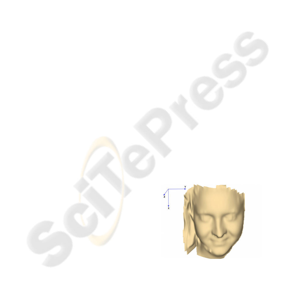
Figure 1: Original 3D mesh with 48,672 vertices and 78,043

faces. The size of the ﬁle (OBJ format) is 4.83MB with

texture mapping and 4.0MB with no texture.

Figure 4 depicts the intersection of all horizontal

and vertical planes where each intersection is marked

SIGMAP 2010 - International Conference on Signal Processing and Multimedia Applications

132

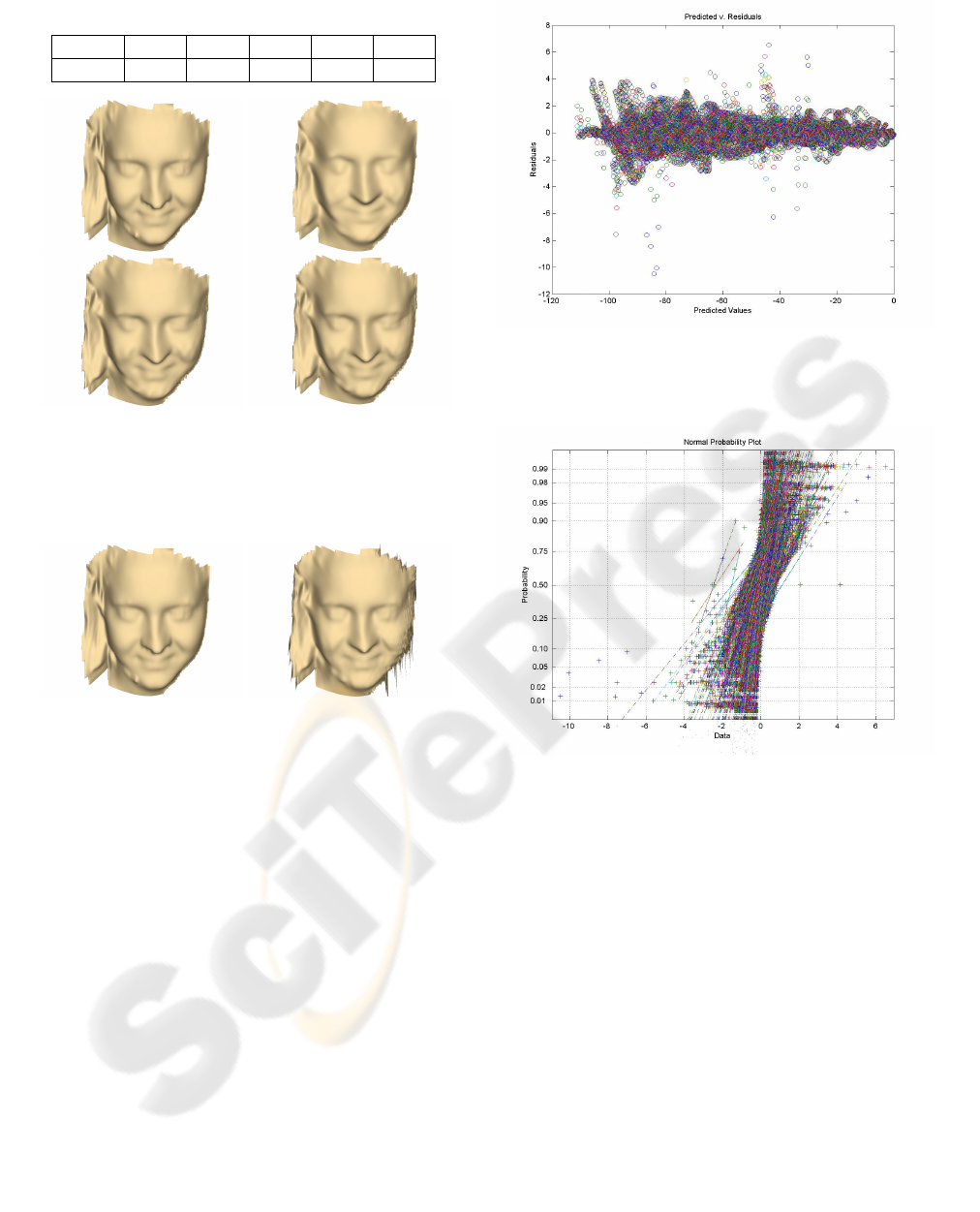
Table 1: Compression rates in percentage.

Degree 20 30 40 50 80

Rate 99.35 99.07 98.79 98.53 97.66

Figure 5: Top row: the original face model is shown on the

left with ﬁle size of 4MB; right, with polynomial interpo-

lation of degree 20 reducing the ﬁle size to 26KB. Bottom

row: left, polynomial interpolation of degree 30 reducing

the ﬁle size to 37.2KB; right, degree 40 reducing to 48.5KB.

Figure 6: Left, the original face model; right, interpolation

with polynomial degree 80. It is noted that the model be-

comes unstable.

3.3 Evaluating the Fit

Determining the quality of a polynomial regression or

how well the recovered data points ﬁt the original data

can involve a number of tests including statistics sum-

maries. By far the most meaningful way is by plotting

the original and regression data sets and visually as-

sess its quality. By visually analyzing the models of

Figure 5, it is suggested that a polynomial interpola-

tion of degrees 20 to 40 describes well the data and

can be well-suited for most applications.

Another way of assessing quality is to look at the

residuals and plot them against the predicted values.

Figure 7 shows the plot for data interpolated with a

polynomial of degree 30. For a good ﬁt, the plot

should display no patterns and no trends. The scatter

plot shows what looks like random noise which is a

good measure of the quality of the ﬁt. Alternatively, if

the ﬁt is good, a normal-probability plot of the resid-

Figure 7: Scatter plot of Predicted Values against Residuals.

For a good ﬁt, it should show no patterns and no trends. The

plot shows what looks like random noise indicating a good

ﬁt.

Figure 8: The normal-probability plot of the residuals. A

good ﬁt should describe a straight line for each polynomial

curve which is veriﬁed by the plot indicating a good ﬁt.

uals should display a straight line. The plot depicted

in Figure 8 shows that for most polynomials evalu-

ated at each plane, indeed they describe a straight line

indicating a good ﬁt.

There are a number of statistical measures to as-

sess the quality or the appropriateness of a model such

as the coefﬁcient of determination also known as R

that indicates the percent of the variation in the data

that is explained by the model. This can be estimated

by ﬁrst calculating the deviation of the original data

set which gives a measure of the spread. While the to-

tal variation to be accounted for (SST) is given by the

sum of deviation squared, the variation that is not ac-

counted for is the sum of the residuals squared (SSE).

The variation in the data explained by the model is

given by

SIGMAP 2010 - International Conference on Signal Processing and Multimedia Applications

134

= 1 −

SSE

SST

(8)

expressed as percentage. The R

values for some in-

terpolated models are described in Table 2. The ta-

ble shows a trend of increasing R

as the polynomial

degree increases, peaking at around degree 30. For

higher degrees, R

decreases monotonically, and this

is also conﬁrmed by visual inspection of the 3D re-

constructed models whose quality deteriorates as they

become unstable for high degree polynomials.

Table 2: The coefﬁcients of determination R

for polyno-

mial ﬁts of degrees 20–80 for the given data.

Degree 20 30 40 50 80

0.9995 0.9996 0.9995 0.9994 0.9909

4 CONCLUSIONS

We have presented a new method of data compres-

sion applied to surface patches that can be deﬁned as a

single valued function. This is the case of 3D data ac-

quired using standard 3D scanning technologies. The

method was described based on mesh cutting planes

oriented with the global coordinate system with con-

stant step. The points where the plane intersections

intersect the mesh are sampled and this automatically

allows the recovery of all (x, y) coordinates for all

vertices. The z-values are subject to polynomial in-

terpolation of various degrees. Results demonstrate

that the method is effective and can reduce the mesh

over 99%. Both close visual inspection and statisti-

cal measures demonstrate that optimal performance is

achieved for polynomials of degree between 20 to 40

– it seems that the optimal value is around 30, but this

obviously depends on the characteristics of the data.

There seems to be intrinsic limitations using poly-

nomials to approximate complex real world surface

patches. In the future we will investigate the use of

splines as it is possible to get more accurate results

than with polynomials but the price we pay is that it

will generate larger ﬁles as we need to keep the coef-

ﬁcients of all polynomials between the control points.

A more promising approach is to investigate the use of

PDEs and research is under way and will be reported

in the near future.

REFERENCES

3DCT (2010). 3D Compression Technologies Inc. available

at http://www.3dcompress.com/web/default.asp

Brink, W., A. Robinson, and M. Rodrigues (2008). Indexing

Uncoded Stripe Patterns in Structured Light Systems

by Maximum Spanning Trees, British Machine Vision

Conference BMVC 2008, Leeds, UK, 1–4 Sep 2008

Hill, F. S. Jr (2001). Computer Graphics Using OpenGL,

2nd edition, Prentice-Hall Inc, 922pp.

Hollinger, S. Q., A. B. Williams, and D. Manak (2010).

3D data compression of hyperspectral imagery using

vectorquantization with NDVI-based multiple code-

books, available at http://sciencestage.com

Lahanas, M. (2010). Optimal Oriented Bounding Boxes,

http://www.mlahanas.de/CompGeom/opt bbox.htm,

last accessed April 2010.

Rodrigues, M. A. and A. Robinson (2010). Novel Methods

for Real-Time 3D Face Recognition, 6th Annual In-

ternational Conference on Computer Science and In-

formation Systems, 25–28 June 2009, Athens, Greece.

Rodrigues, M. A., A. Robinson, and W. Brink (2008). Fast

3D Reconstruction and Recognition, in New Aspects

of Signal Processing, Computational Geometry and

Artiﬁcial Vision, 8th WSEAS ISCGAV, Rhodes, 2008,

p15–21.

Robinson, A., L. Alboul and M. A. Rodrigues (2004). Meth-

ods for Indexing Stripes in Uncoded Structured Light

Scanning Systems, Journal of WSCG, 12(3), 2004, pp

371–378.

Szymczak, A., D. King and J. Rossignac (2000). An

Edgebreaker-Based Efﬁcient Compression Scheme

for Regular Meshes, 12th Canadian Conference on

Computational Geometry, pp 257–265.

Szymczak, A., J. Rossignac, and D. King (2002), Piecewise

Regular Meshes, Graphical Models 64(3-4), 2002,

183–198.

Shikhare, D., S. V. Babji, and S. P. Mudur (2002). Com-

pression techniques for distributed use of 3D data: an

emerging media type on the internet, 15th interna-

tional conference on Computer communication, India,

pp 676–696.

EFFICIENT 3D DATA COMPRESSION THROUGH PARAMETERIZATION OF FREE-FORM SURFACE PATCHES

135