POWER CONSUMPTION-BASED AND TRANSMISSION

RATE-BASED ALGORITHMS IN COMMUNICATION-BASED

NETWORK APPLICATIONS

Tomoya Enokido

Faculty of Bussiness Administration, Rissho University, Tokyo, Japan

Ailixier Aikebaier, and Makoto Takizawa

Department of Computers and Information Science, Seikei University, Musashino-shi, Tokyo, Japan

Keywords:

Green IT, Power consumption, Communication-based systems, Power Consumption-Based (PCB) algorithm,

Transmission Rate-Based (TRB) algorithm.

Abstract: In order to realize eco societies, we have to reduce the total electrical power consumption in information

systems. We classify network applications into transaction and communication based applications. CPU

resources of servers are mainly consumed in the transaction based ones. In this paper, we consider com-

munication based applications where a server transmits a large volume of data to a client like ﬁle transfer

protocol (FTP). We discuss a power consumption model for communication-based applications. In the model,

the total power consumption of a server depends on the total transmission rate and number of clients where

the server concurrently transmits ﬁles. A client has to select a server in a set of possible servers, each of

which holds a ﬁle, so that the power consumption of the server is reduced. We newly discuss a pair of PCB

(power consumption-based) and TRB (transmission rate-based) algorithms to select a server. In the evalua-

tion, we show the total power consumption can be reduced by the PCB and TRB algorithms compared with

the traditional round-robin (RR) algorithm and PCB is more practical than TRB.

1 INTRODUCTION

In the green IT technologies (Green IT, 2010), the to-

tal electric power consumption of computers and net-

works has to be reduced. Various types of hardware

technologies like low-power consumption CPUs and

storages are now being developed. A cloud comput-

ing system (Grossman, 2009; Zhang and Zhou, 2009)

is composed of a huge number of server computers

like Google ﬁle systems (Ghemawat et al., 2003).

Biancini et al. (Bianchini and Rajamony, 2004) dis-

cuss how to reduce the power consumption of a clus-

ter of homogeneous servers by turning off servers

which are not required for executing a collection of

web requests. Various types of algorithms to ﬁnd re-

quired number of servers in homogeneous and het-

erogeneous servers are discussed (Heath et al., 2005;

Rajamani and Lefurgy, 2003; Aikebaier et al., 2009;

Yang et al., 2009b). In wireless sensor networks

(Akyildiz and Kasimoglu, 2004; Yang et al., 2009a),

routing algorithms (Zhao et al., 2010) to reduce the

power consumption of the battery in a sensor node

are discussed.

There are transaction-based and communication-

based network applications. We discussed how to

reduce the power consumption in transaction-based

applications like Web applications (Aikebaier et al.,

2009; Enokido et al., 2010b; Enokido et al., 2010a;

Yang et al., 2009b). Clients issue Web requests to

servers. Then the servers encode multimedia con-

tents and send replies with the encoded contents to the

clients. We assume the communication bandwidth is

inﬁnite, i.e. the communication overhead is so small

as to be neglected compared with the processing over-

head of servers, mainly for encoding multimedia ob-

jects. In another type of application like the ﬁle trans-

fer protocol (FTP), a large volume of data is trans-

mitted by a server to a client. According to our ex-

periments, the power consumption of the server to

transmit a ﬁle to a client depends on the transmis-

sion rate of the server. First, a client ﬁnds a server

which holds a ﬁle so that not only the time constraints

Enokido T., Aikebaier A. and Takizawa M. (2010).

POWER CONSUMPTION-BASED AND TRANSMISSION RATE-BASED ALGORITHMS IN COMMUNICATION-BASED NETWORK APPLICATIONS.

In Proceedings of the Multi-Conference on Innovative Developments in ICT, pages 13-22

DOI: 10.5220/0003034800130022

 SciTePress

are satisﬁed but also the power consumption of the

server is reduced. In this paper, we discuss a power

consumption model for transmitting ﬁles based on the

experimental results. We newly discuss a pair of PCB

(power consumption-based) and TRB (transmission

rate-based) algorithms to select a server in a set of

servers so that the total power consumption can be

reduced. We evaluate the PCB and TRB algorithms

in terms of the total power consumption and the to-

tal transmission time compared with the traditional

round-robin (RR) algorithm (Weighted Least Connec-

tion (WLC), 1998; Weighted Round Robin (WRR),

1998). We show the total power consumption and

the total transmission time can be reduced in the PCB

and TRB algorithms. The TRB algorithm is based

on the transmission rate but it is difﬁcult to estimate

the bandwidth since the transmission rate is in reality

changed in the networks. Hence, the PCB algorithm

is more useful than the others since the transmission

rate is not considered.

In section 2, we discuss a model of ﬁle transmis-

sion. In section 3, we show the experimental results

of the total power consumption in ﬁle transfer ap-

plications and then discuss the power consumption

model. In section 4, we discuss how to select a server

for downloading a ﬁle to reduce the power consump-

tion. In section 5, we evaluate the PCB and TRB al-

gorithms compared with the RR algorithm.

2 FILE TRANSFER MODEL

Suppose there are a collection S = {s

, ..., s

} of

servers, where each server s

holds a full replica of

a ﬁle f. A client c

selects one server s

in the server

set S and issues a transmission request to the server s

Then, the server s

transmits the ﬁle f to the client c

as shown in Figure 1.

server client

Figure 1: File transfer model.

Suppose a server s

concurrently sends ﬁles f

, ...,

to a set C

of clients c

, ..., c

at rates tr

(τ), ...,

(τ) (m ≥ 1), respectively, at time τ. b

shows the

maximum bandwidth [bps] between a server s

and a

client c

. Let Maxtr

be the maximum transmission

rate [bps] of the server s

(≤ b

) which is smaller

than the bandwidth b

of the network. Here, the to-

tal transmission rate tr

(τ) of the server s

at time τ

is given as tr

(τ) = tr

(τ) + ··· + tr

(τ). Here, 0 ≤

(τ) ≤ Maxtr

Each client c

receives messages at receipt rate

(τ) at time τ. Let Maxrr

indicate the maximum

receipt rate of the client c

. Here, tr

(τ) ≤ Maxrr

We assume each client c

receives a ﬁle from at most

one server at rate Maxrr

(= rr

(τ)). The server s

al-

locates each client c

with transmission rate tr

(τ) so

that tr

(τ) ≤ Maxrr

at time τ.

Let T

be the total transmission time of a ﬁle

from a server s

to a client c

. If the server

sends ﬁles to other clients concurrently with the

client c

, the transmission time T

is increased. Let

minT

show the minimum transmission time | f

| /

min(Maxrr

, Maxtr

) [sec] of a ﬁle f

from a server

to a client c

where | f

| indicates the size [bit] of

the ﬁle f

. T

≥ minT

The average transmission rate (ATR) A

of the

server s

to the client c

is deﬁned as 1 / T

[1/sec].

Let maxA

be 1 / minT

. maxA

= max(maxA

, ...,

maxA

) and minA

= min(maxA

, ..., maxA

Let tr

(τ) show the transmission rate of a ﬁle f

from the server s

to the client c

at time τ. Sup-

pose the server s

starts and ends transmitting a ﬁle

to the client c

at time st and et, respectively. Here,

(τ) dτ = | f

| and the transmission time T

is et

- st. If the server s

sends only the ﬁle f

to the client

at time τ, tr

(τ) = min(Maxtr

, Maxrr

) [bps].

The laxity l

fts

(τ) is |f

| -

(x) dx [bit] at time

τ, i.e. how many bits of a ﬁle f

the server s

still has

to transmit to the client c

at time τ.

There are types of computers with respect to the

normalized transmission rate (NTR). Let F

(τ) be a set

of current ﬁles which the server s

is transmitting to

clients at time τ. LetC

(τ) be a set of clients c

, ..., c

to which the server s

transmits ﬁles f

, ..., f

in F

(τ),

respectively, at time τ. First, we consider a model

where a server s

satisﬁes the following properties:

[Server-bound Model]. If Maxrr

+ · ·· + Maxrr

≥ Maxtr

, for every time τ,

∑

∈C

(τ)

(τ) = d(τ) ·

maxA

Here, d(τ) (≤ 1) shows the degradation factor

(1−|C

(τ)|)

(0 < γ ≤ 1) at time t. Here, the effective

transmission rate of the server s

is d(τ)·maxA

. The

more number of clients a server concurrently sends

ﬁles, the smaller effective transmission rate.

Let us consider three ﬁles f

, f

, and f

which a

server s

sends to clients c

, c

, and c

as an example.

First, suppose that the server s

serially sends the ﬁles

, f

, and f

to the clients c

, c

, and c

, i.e. et

= st

and et

= st

as shown in Figure 2. Here, the

transmission time T

is et

- st

= minT

t f

+ minT

t f

minT

t f

. Next, suppose the server s

starts transmitting

three ﬁles f

, f

, and f

at time st and terminates at

time et as shown in Figure 2 (2). Here, since three

INNOV 2010 - International Multi-Conference on Innovative Developments in ICT

time τ

maxA

time τ

(1) serial transmission.

(2) parallel transmission.

minT

(

)+ +

maxA

-2

Figure 2: Transmission time.

ﬁles are concurrently transmitted, C

(t) = 3 and γ

−2

= minT

t f

+ minT

t f

+ minT

t f

. For γ = 0.98, it takes

about 1.4% longer time than the serial transmission.

On the other hand, we consider another environ-

ment where a client c

cannot receive a ﬁle from a

server s

at rate Maxtr

, i.e. Maxrr

< Maxtr

. Hence,

the transmission rate tr

of the server s

to a client c

is Maxrr

[Client-bound model]. If Maxrr

+ ··· + Maxrr

≤ Maxtr

∑

∈C

(τ)

(τ) = maxA

· (Maxrr

+ ··· +

Maxrr

) / Maxtr

Even if every client c

receives a ﬁle at maximum

rate Maxrr

, the effective transmission rate is not de-

graded.

3 EXPERIMENTAL RESULTS

AND POWER CONSUMPTION

MODEL

3.1 Environment

We measure how much electric power a computer

spends to transfer ﬁles to other computers by using

the powermeter Watts up?.Net (Watts up? .Net, 2009)

where the power consumption of each computer can

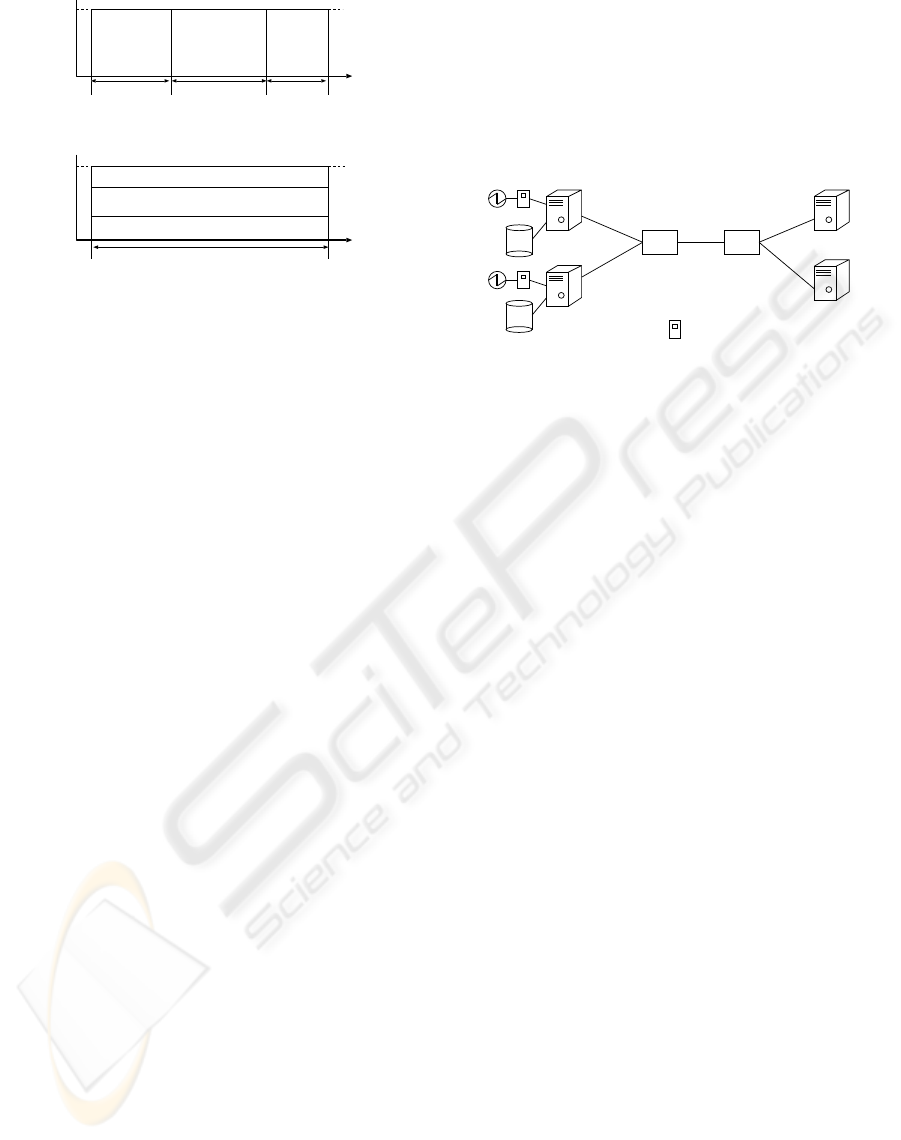
be measured every one second. As shown in Figure 3,

a pair of server computers s

and s

are interconnected

with a pair of client computers c

and c

in 1Gbps net-

works. Table 1 summarizes the speciﬁcations of the

servers s

and s

. The server s

is equipped with a

one-core CPU. The server s

is composed of a pair

of two-core CPUs. That is, the bandwidth b

from a

server s

to a client c

is 1Gbps (t = 1, 2). Each client

downloads a ﬁle f from one of the servers. The

size of the ﬁle f is 43,051,806 bytes long. Here, we

measure the total power consumption of the servers s

and s

For each server s

, we consider two types of ex-

perimentations, one-client (1C

) and two-client (2C

)

environments (t = 1, 2). In the 1C

environment, one

client, say c

downloads the ﬁle f from the server s

In the 2C

environment, a pair of the clients c

and c

concurrently download the ﬁle f from the server s

1Gbps

1Gbit

switch

servers

1Gbps

1Gbit

switch

1Gbps

clients

1Gbps

: meter.

Figure 3: Experimental environment.

3.2 Power Consumption

A server s

consumes the electric power to transmit

ﬁles to clients while clients consume less amount of

electric power. The power consumption rate shows

the electric power consumption for a second [W/sec].

In the 1C

environment, the server s

transmits a ﬁle

f to one client, say c

at rate tr

. Here, the server

is composed of one one-core CPU. The maximum

transmission rate Maxtr

is 160 [Mbps] in the net-

work of bandwidth b

= 1G [bps]. In the 2C

en-

vironment, the server s

concurrently transmits the

ﬁle f to a couple of clients c

and c

. Here, tr

+ tr

. Figure 4 shows the power consumption

rate of the server s

for the total transmission rate

. At the higher rate tr

the server s

transmits the

ﬁle f, the larger amount of power consumption the

server s

consumes. We obtain the approximated for-

mula PC

(tr) to show the power consumption rate of a

server s

for total transmission rate tr [Mbps] by using

the least-squares method to the experimental results.

In Figure 4, the bold dotted line shows the approxi-

mated power consumption of the server s

where one

client downloads the ﬁle f from the server s

. The

dotted line shows the approximated power consump-

tion of the server s

where a pair of clients c

and c

concurrently download the ﬁle f from the server s

Let PC

(tr) and PC

(tr) be the power consumption

rates in the 1C

and 2C

environments, respectively,

at total rate tr.

: PC

(tr) = 0.11tr + 4.15 [W/sec].

: PC

(tr) = 0.12tr + 4.43 [W/sec].

In a single-CPU server s

, the power consumption

rate PC

(tr) is proportional to the total transmission

rate tr.

Next, we consider another server s

which is com-

posed of a pair of two-core CPUs. Here, the maxi-

POWER CONSUMPTION-BASED AND TRANSMISSION RATE-BASED ALGORITHMS IN

COMMUNICATION-BASED NETWORK APPLICATIONS

Table 1: Servers.

Server s

Number of CPUs 1 2

Number of cores / CPU 1 2

CPU AMD Athlon 1648B (2.7GHz) AMD Opteron 270 (2GHz)

Memory 4,096MB 4096MB

DISK 150GB 7200rpm 74GB 10000rpm x 2 RAID1

NIC Broadcom Gbit Ether (1Gbps) Nvidia Ether Controler (1Gbps)

0 20 40 60 80 100 120 140 160

Power consumption rate [W/sec].

Total transmission rate tr [Mbps].

1 CPU (1 core) and 1C

1 CPU (1 core) and 2C

0.11tr+4.15

0.12tr+4.43

Figure 4: One-CPU : Power consumption rate [W/sec].

mum transmission rate Maxtr

of the server s

is 450

[Mbps]. We measure the power consumption rate for

the total transmission rate tr

for 1C

and 2C

. Fig-

ure 5 shows the power consumption rate [W/sec] of

the server s

for the total transmission rate tr. Follow-

ing Figure 5, the power consumption rate of the server

also depends on the total transmission rate tr

. At the higher rate the server s

transmits, the

larger power consumption s

consumes. The approx-

imated formulas PC

(tr) and PC

(tr) of the power

consumption rate of the server s

for total transmis-

sion rate tr [Mbps] are given in the 1C

and 2C

en-

vironments as follows:

: PC

(tr) = 0.02tr + 3.02 [W/sec].

: PC

(tr) = 0.03tr + 3.34 [W/sec].

The increase rate of the power consumption of the

server s

in 2C

is about 1.5 times larger than 1C

Compared with the one-CPU case 1C

, the power con-

sumption rate is not so much increased for the in-

crease of transmission rate in the two-CPU case 2C

Following the experiments, the power consump-

tion rate PC

(tr) of a server s

is lineally increased for

transmission rate tr (0 ≤ tr ≤ Maxtr

) as follows:

(tr) = β

(m) · α

·tr+ minE

. (1)

Here, α

is the power consumption to transmit one

Mbits [W/Mb] for the 1C

environment. α

depends

on a server type s

. As shown in Figures 4 and 5, the

more number of clients, the more amount of electric

power is consumed. β

(m) shows how much power

0 50 100 150 200 250 300 350 400 450

Power consumption rate [W/sec].

Total transmission rate tr [Mbps].

2 CPU (4 core) and 1C

2 CPU (4 core) and 2C

0.02tr+3.02

0.03tr+3.34

Figure 5: Two-CPU : Power consumption rate [W/sec].

consumption is increased for the number m of clients,

(m) ≥ 1 and β

(m) ≥ β

(m - 1). There is a ﬁxed

point maxm

such that β

(maxm

- 1) ≤ β

(maxm

) =

(maxm

+ h) for h > 0. minE

gives the minimum

power consumption rate of the server s

where no ﬁle

is transmitted. β

(maxm

)·α

·Maxtr

+ minE

gives

the maximum power consumption rate maxE

of the

server s

Power consumption rate [W/sec]

Total transmission rate tr [Mbps]

minE

Maxtr

maxE

PC (tr) = β (m) α tr + minE

t t t t

Figure 6: Power consumption rate of server s

[W/sec].

3.3 Power Consumption Model

We would like to discuss how much electrical power

a server s

consumes to transfer a ﬁle to a client c

Suppose there are n (≥ 1) servers s

,... ,s

, each of

which holds a ﬁle f. Let E

(τ) show the electric power

consumption rate of a server s

at time τ [W/sec] (τ =

1,...,n). maxE

and minE

indicate the maximum and

INNOV 2010 - International Multi-Conference on Innovative Developments in ICT

minimum electric power consumption of a server s

respectively. Here, minE

shows the power consump-

tion of a server s

which is in idle state. That is, minE

≤ E

(τ) ≤ maxE

. maxE and minE show max(maxE

..., maxE

) and min(minE

, ..., minE

), respectively.

In this paper, we assume that only ﬁle transfer ap-

plications are performed on each server. The electric

power consumption rate E

(τ) of a server s

at time τ

is given as follows:

(τ) = PC

(tr

(τ)). (2)

As discussed in the preceding section, E

(τ) is

given in a linear function (1). E

(τ) = β

(|C

(τ)|) · α

(τ) + minE

. Here, C

(τ) indicates a set of clients to

which a server s

sends ﬁles at time τ.

The power consumption TPC

(τ

,τ

) [W] of a

server s

from time τ

to time τ

is given as follows:

TPC

(τ

,τ

) =

(τ)dτ. (3)

4 SELECTION ALGORITHMS OF

SERVERS

4.1 System Model

There are a set S of multiple servers s

, ..., s

, each of

which holds a full replica of a ﬁle f. A client c

sends

a transfer request of the ﬁle f to a load balancer K.

Then, the load balancer K selects one server s

in the

set S. The server s

transmits the ﬁle f to the client

. We discuss how to select a server in the set S for a

client c

so that the following constraints are satisﬁed:

1. The ﬁle f has to be transmitted to the client so as

to satisfy the deadline constraint.

2. The power consumption of a selected server s

transfer the ﬁle f has to be minimized.

load balancer

Figure 7: FTP model.

4.2 Round-robin Algorithms

In a load balancer K, types of round-robin algorithms

are widely used. In the basic round-robin (RR) al-

gorithm, the servers s

, ..., s

in the server set S are

totally ordered. A request is ﬁrst issued to the ﬁrst

server s

in the ordered set. If s

is overloaded, a re-

quest is sent to the second server s

. Thus, if servers

, ..., s

are overloaded, a request is issued to a server

i+1

(i < n).

We further consider weighted round robin (WRR)

(Weighted Round Robin (WRR), 1998) and weighted

least connection (WLC) (Weighted Least Connection

(WLC), 1998) algorithms. For each of the WRR and

WLC algorithms, we consider two cases, Per (perfor-

mance) and Pow (power). In Per, the weight is given

in terms of the performance ratio of the servers. That

is, the higher performance a server supports, the more

number of processes are allocated to the server. On

the other hand, the weight is deﬁned in terms of the

power consumption rate of the servers in Pow. The

smaller power a server consumes, the more number

of processes are allocated to the server.

4.3 Algorithm for Allocating

Transmission Rates

At time τ, the maximum transmission rate maxtr

(τ)

of a server s

depends on the degradation factor d

(τ)

of the server s

, i.e. the number of clients to which the

server s

concurrently transmits ﬁles at time τ. Each

time a new request is issued by a client c

and a cur-

rent request for a client c

is terminated at time τ,C

(τ)

= C

(τ) + {c

} and C

(τ) = C

(τ) - {c

}, respectively.

Here, the maximum transmission rate maxtr

(τ) of a

server s

at time τ is calculated as γ

1−|C

(τ)|

· Maxtr

Here, 0 < γ ≤ 1. The transmission rate tr

(τ) of a

server s

for a client c

at time τ is calculated as fol-

lows:

CalcMAXTR

TS(s

, c

, τ) {

check = False;

maxtr

(τ) = γ

1−|C

(τ)|

· Maxtr

;

nc = |C

(τ)| + {c

};

/*C

(τ) is sorted in ascending order of Maxrr

.*/

SORT(C

(τ));

for each c

in C

(τ) {

/*take a client c

in the ascending order.*/

if Maxrr

≤ maxtr

(τ) / nc, {

if c

= c

, {

(τ) = Maxrr

;

maxtr

(τ) = maxtr

(τ) - tr

(τ);

check = True;

break;

}

POWER CONSUMPTION-BASED AND TRANSMISSION RATE-BASED ALGORITHMS IN

COMMUNICATION-BASED NETWORK APPLICATIONS

(τ) = maxtr

(τ) - Maxrr

;

maxtr

(τ) = maxtr

(τ) - tr

(τ);

nc = nc - 1;

}

} /* for end */

if check = False, {

(τ) = maxtr

(τ) / nc;

break;

}

return(tr

(τ));

}

In the procedure CalcMAXTR TS(), each server

can transmit a ﬁle at least tr

(τ) = maxtr

(τ) /

(τ)| [Mbps] to a client c

in the set C

(τ). Here,

if the maximum receipt rate Maxrr

(τ) of a client c

larger than the maximum transmission rate maxtr

(τ)

allocated for a client c

, the server s

transmits a ﬁle

to the client c

at rate tr

(τ) at time τ. Otherwise, the

server s

transmits at rate maxrr

(τ). Here, the unused

part of the maximum transmission rate of the server s

for the client c

(= tr

(τ) - maxrr

(τ)) can be used for

other clients.

Suppose a server s

is selected by three clients c

, c

(τ) = {c

, c

}) and the maximum trans-

mission rate maxtr

(τ) of the server s

is 6 [Mbps] at

time τ as shown in Figure 8. Suppose Maxrr

= 1

[Mbps], Maxrr

= 2 [Mbps], and Maxrr

= 3 [Mbps].

In the basic fair allocation algorithms, each client c

is allocated with the same transmission rate tr

(τ) =

maxtr

(τ) / |C

(τ)| = 6 / 3 = 2 [Mbps] as shown in Fig-

ure 8 (1). Here, the transmission rate 2 - 1 = 1 [Mbps]

is not used for the client c

. In addition, the client

cannot use the maximum receipt rate Maxrr

(= 3

[Mbps]). On the other hand, the unused transmission

rate of the client c

(= 1 [Mbps]) can be used for the

client c

in the procedure CalcMAXTR TS(). Then,

each client c

(s = 1, 2, 3) can download ﬁles from the

server s

at the maximum receipt rate Maxrr

at time

τ.

4.4 Selection Algorithms

Next, we discuss how a load balancer K selects a

server s

for a client c

in the server set S. In

this paper, we propose two novel allocation algo-

rithms, transmission rate-based (TRB) and power

consumption-based (PCB) algorithms to select a

server for a client. In the TRB algorithm, a server s

is selected for a client c

where the transmission rate

(τ) of the server s

to transmit a ﬁle f to a client

is the largest. The TRB algorithm is shown as fol-

lows:

maxtr (t) = 6

maxtr (t) = 2

maxtr (t) = 1

maxtr (t) = 2

maxtr (t) = 3

(1) basic fair allocation. (2) CalcMAXTR_TS() procedure.

Figure 8: Transmission rate allocation.

TRB(c

, τ) {

server = φ; MAXTR = 0;

for each s

in S {

(τ) = CalcMAXTR

TS(s

, c

, τ);

if server = φ, {

server = s

;

MAXTR = tr

(τ);}

else {

if MAXTR < tr

(τ), {

MAXTR = tr

(τ);

server = s

;

}

return(server);

}

In the PCB algorithm, a server s

is selected for the

client c

where the power consumption to transmit a

ﬁle f to a client c

is the smallest. Here, | f| / tr

(τ)

is an estimated transmission time at time τ when a

server s

starts transmitting a ﬁle f to a client c

with

a transmission rate tr

(τ). The power consumption

rate E

(τ) of each server s

at time τ is β

(|C

(τ)|) · α

· tr

(τ) as discussed in the preceding section. It is not

easy to estimate how much electric power the server

consumes to transmit a ﬁle f to the client c

since

there might be other clients which receive ﬁles. Here,

the estimated change of power consumption EE

(τ)

[W] of a server s

for transmitting a ﬁle f to a client

at time τ when s

starts transmitting f is deﬁned as

follows:

(τ)

= (| f| / tr

(τ)) · β

(|C

(τ)|) · α

·tr

(τ)

= | f| · β

(|C

(τ)|) · α

(4)

Here, a server s

is selected for a client c

in the PCB

algorithm by using EE

(τ) at time τ as follows:

PCB(c

, τ) {

server = φ; EPC = 0;

for each s

in S {

EPC

(τ) = | f| · β

(|C

(τ)|) · α

if server = φ, {

server = s

;

INNOV 2010 - International Multi-Conference on Innovative Developments in ICT

EPC = EE

(τ);}

else {

if EPC > EE

(τ), {

EPC = EE

(τ); server = s

;

}

return(server);

}

For example, there are a pair of servers s

and

. The maximum transmission rates of the servers

and s

are 7 [Mbps] and 6 [Mbps], respectively,

i.e. Maxtr

= 7 [Mbps] and Maxtr

= 6 [Mbps]. The

power consumption coefﬁcients α

and α

to trans-

mit one [Mbit] for one client of servers s

and s

are

0.10 and 0.03, respectively. A server s

is selected by

two clients c

and c

(τ) = {c

, c

}) and an-

other server s

is selected by two clients c

and c

(τ) = {c

, c

}) at time τ, respectively. The maxi-

mum receipt rates of clients c

and c

are the same 1

[Mbps] (Maxrr

= Maxrr

= 1 [Mbps]). The maxi-

mum receipt rates of clients c

and c

are the same

2 [Mbps] (Maxrr

= Maxrr

= 2 [Mbps]). Suppose

a client c

issues a new request to transmit a ﬁle f

whose size is ten Mbytes to a load balancer K at time

τ. Here, the maximum receipt rate Maxrr

for the ﬁle

f on the client c

is 4 [Mbps]. According to the pro-

cedure CalcMAXTR TS(···), the unused transmis-

sion rates of the servers s

and s

are 4 [Mbps] and 3

[Mbps], respectively. The servers s

and s

can allo-

cate transmission rates 4 [Mbps] and 3 [Mbps] for the

client c

, respectively. In the TRB algorithm, a server

which can allocate the maximum transmission rate

to a client c

is selected. Therefore, the server s

selected for a client c

. On the other hand, a server

which has the minimum value of the formula | f| ·

(|C

(τ)|) · α

is selected in the PCB algorithm, i.e. a

server which can mostly save the power consumption

is selected at time τ. Here, sets C

(τ) and C

(τ) of cur-

rent clients of servers s

and s

include three clients,

respectively. Suppose the increasing rates β

(3) and

(3) of the power consumption of the servers s

and

are 1.2 and 1.09, respectively. Here, | f|·β

(3)·α

10 · 1.2 · 0.10 = 1.2. | f|·β

(3)·α

= 10 · 1.09 · 0.03 =

0.327. Therefore, the server s

is selected for a client

in the PCB algorithm.

5 EVALUATION

5.1 Evaluation Environment

We evaluate the TRB and PCB algorithms in terms

of the total amount of power consumption and total

transmission time of ﬁles compared with the basic RR

algorithm through the simulation. In the evaluation,

there are ﬁve servers s

, s

, and s

as shown in

Table 2, S = {s

, s

}. The power consump-

tion coefﬁcient α

to transmit one Mbits for one client

of each server s

is randomly selected between 0.02

and 0.11 [W/Mb] based on the experimental results.

The increasing rate of the power consumption β

(m)

for the number m of clients is randomly selected be-

tween 1.09 and 1.5. The minimum power consump-

tion rate minE

of each server s

is randomly selected

between 3 and 4 [W]. The maximum transmission rate

Maxtr

of each server s

is randomly selected between

150 and 450 [Mbps]. Each server s

has a replica of a

ﬁle f. The size of the ﬁle f is one giga-byte.

Totally 100 clients download the ﬁle f from one

server s

in the server set S. The maximum receipt

rate Maxrr

of each client c

is randomly selected be-

tween 0.1 and 100 [Mbps]. Each client c

issues a

transfer request of the ﬁle f to a load balancer K at

time st

. Here, the starting time st

of each client c

is randomly selected between 1 and 3,600 [sec] at the

simulation time. Each client c

issues one request at

time st

in the simulation. In the simulations of the

TRB, PCB, and RR algorithms, the starting time st

of the ﬁle transmission to each client c

is the same.

Table 2: Types of servers.

Servers α β(m) minE [W] Maxtr [Mbps]

0.03 1.259 3.39 406

0.05 1.195 3.17 401

0.03 1.285 3.12 249

0.09 1.117 3.90 231

0.02 1.162 3.02 171

5.2 Total Power Consumption

Figure 9 shows the total power consumption rate

[W/sec] of the servers s

, ..., s

at each time. Table 3

shows the total power consumptions of the servers in

the PCB, TRB, and RR algorithms. The total power

consumptions of the PCB, TRB, and RR algorithms

are 546,186 [W], 654,161 [W], and 1,073,914 [W],

respectively. In the PCB algorithm, the total amount

of power consumption is the smallest because a server

is selected for a client c

, whose the power con-

sumption is the smallest to transmit a ﬁle f to the

client c

. In the TBR algorithm, a server s

is selected

for a client c

, whose transmission rate for the client

is the largest. Then, the total amount of power con-

sumption is larger than the PCB algorithm. On the

other hand, the total amount of power consumption of

the TRB algorithm is smaller than the RR algorithm.

POWER CONSUMPTION-BASED AND TRANSMISSION RATE-BASED ALGORITHMS IN

COMMUNICATION-BASED NETWORK APPLICATIONS

Table 3: Total amount of power consumption.

PCB TRB RR

546,186 [W] 654,161 [W] 1,073,914 [W]

0 10000 20000 30000 40000 50000

Power consumption per sec [W/sec]

Simulation time [sec]

PCB algorithm

TRB algorithm

RR algorithm

Figure 9: Total power consumption rate.

5.3 Total Transmission Time

Table 4 shows the total transmission time of the ﬁles

to the 100 clients in the PCB, TRB, and RR algo-

rithms. The total transmission time are 28,614 [sec],

28,594 [sec], and 43,744 [sec] in the PCB, TRB, and

RR algorithms, respectively. The total transmission

time of the TRB algorithm is smaller than the PCB

and RR algorithms. However, the difference of the

total transmission time between TRB and PCB is ne-

glectable. In the TRB algorithm, a server s

is se-

lected, which can supply the maximum transmission

rate. Therefore, the difference of the transmission

time between PCB and TRB is so small as to be ne-

glected in this simulation.

Table 4: Total transmission time of the ﬁles.

PCB TRB RR

28,614 [sec] 28,594 [sec] 43,744 [sec]

In the PCB algorithm, a server s

is selected for

a client c

without considering the transmission rate

between the server s

and the client c

. On the other

hand, a server s

is selected for a client c

based on

the estimated transmission rate in the TRB algorithm.

From the evaluation results, we consider the total

power consumption can be more reduced in the PCB

algorithm than the TRB algorithm and the difference

of the total transmission time between the PCB and

TRB algorithms is neglectable. In reality, the trans-

mission rate between a server s

and a client c

is dy-

namically changed in the network since the transmis-

sion rate of a server s

is dynamically changed based

on the number of clients. It is not easy to estimate the

transmission rate of the server s

to a client c

from

the practical point of view. In addition, a server s

for a client c

can be selected without considering the

transmission rate between the server s

and the client

in the PCB algorithm. Therefore, the PCB algo-

rithm is simpler and more useful than the TRB and

RR algorithms.

5.4 File Size

We measured the total transmission time [sec] and the

total power consumption of the PCB, TRB, and RR

algorithms to transmit ﬁve types of ﬁles whose sizes

are 1, 2, 3, 4, and 5 [GB], respectively. Totally the 100

clients download the ﬁle f from one s

of the servers

in the server set S (= {s

, s

}). Table 5

and Figure 10 show the total transmission time in the

PCB, TRB, and RR algorithms for each ﬁle size. The

total transmission time of the RR algorithm is longer

than the PCB and TRB algorithms.

Figure 11 shows the total transmission time in the

PCB and TRB algorithms for ﬁle size. The total trans-

mission time of the TRB algorithm is smaller than the

PCB and RR algorithms. The difference of the total

transmission time between the PCB algorithm and the

TRB algorithm is almost neglectable.

Table 5: Total transmission time [sec].

PCB TRB RR

1GB 28,614 28,594 43,744

2GB 55,599 55,521 430,248

3GB 82,585 82,354 1,722,061

4GB 109,570 108,958 4,570,858

5GB 136,556 135,036 7,276,956

1 2 3 4 5

Total transmission time [sec]

File size [GB]

PCB algorithm

TRB algorithm

RR algorithm

[x 10 ]

Figure 10: Total transmission time (PCB, TRB, and RR).

Next, we measured the total power consumption

[W] of the ﬁve servers s

, ..., s

in the PCB, TRB, and

RR algorithms. Table 6 and Figure 12 show the total

INNOV 2010 - International Multi-Conference on Innovative Developments in ICT

1 2 3 4 5

Total transmission time [sec]

File size [GB]

PCB algorithm

TRB algorithm

[x 10 ]

Figure 11: Total transmission time (PCB and TRB).

amount of power consumption in the PCB, TRB, and

RR algorithms for each ﬁle size. Figure 13 shows the

total amount of power consumption of the servers in

the PCB and TRB algorithms. The total amount of

power consumption of the PCB algorithm is smaller

than the TRB and RR algorithms. The total amount of

power consumption of the TRB algorithm is smaller

than the RR algorithm. The PCB algorithm is better

than the TRB and RR algorithms for any ﬁle size.

Table 6: Total power consumption [W].

PCB TRB RR

1GB 546,186 654,161 1,073,914

2GB 1,209,621 1,405,971 10,647,775

3GB 1,971,767 2,215,575 42,670,592

4GB 2,835,375 3,131,209 113,334,809

5GB 3,998,291 4,211,034 180,500,814

1 2 3 4 5

Total power consumption [W]

File size [GB]

PCB algorithm

TRB algorithm

RR algorithm

[x 10 ]

Figure 12: Total power consumption (PCB, TRB, and RR).

1 2 3 4 5

Total power consumption [W]

File size [GB]

PCB algorithm

TRB algorithm

[x 10 ]

Figure 13: Total power consumption (PCB and TRB).

6 CONCLUDING REMARKS

In this paper, we discussed how much electric power a

server consumes to transfer a ﬁle to a client. A server

consumes the electric power proportional to the trans-

mission rate. Through the experiments, we obtained

approximate linear functions showing how much a

server computer consumes the electric power to trans-

mit ﬁles to clients for transmission rate. We proposed

the PCB and TRB algorithms to select a server so that

the total power consumption of the servers is reduced.

We evaluated the PCB and TRB algorithms in terms

of the total power consumption and the total trans-

mission time compared with the basic RR algorithm

through simulation. According to the evaluation re-

sults, the total power consumption and the total trans-

mission time can be reduced in the PCB and TRB al-

gorithms compared with the basic RR algorithm. In

the PCB algorithm, the total power consumption can

be more reduced than the TRB algorithm and the dif-

ference of the total transmission time between PCB

and TRB is almost neglectable. It is not necessary to

estimate the transmission rate between a server and

a client in the PCB algorithm. In addition, the total

power consumption and total transmission time are

no increased in the PCB and TRB algorithms com-

pared with the RR algorithm even if the ﬁle size is

increased. Therefore, the PCB algorithm is more use-

ful for reducing the total power consumption in the

communication-based applications.

REFERENCES

Aikebaier, A., Enokido, T., and Takizawa, M. (2009).

Energy-efﬁcient computation models for distributed

systems. In Proceedings of the 12th International

POWER CONSUMPTION-BASED AND TRANSMISSION RATE-BASED ALGORITHMS IN

COMMUNICATION-BASED NETWORK APPLICATIONS

Conference on Network-Based Information Systems

(NBiS2009), pages 29–36. IEEE CS Press.

Akyildiz, I. F. and Kasimoglu, I. H. (2004). Wireless sensor

and actor networks: Research challenges. In Ad Hoc

Networks journal, volume 2, pages 351–367. Elsevier.

Bianchini, R. and Rajamony, R. (2004). Power and energy

management for server systems. In IEEE Computer,

volume 37(11), pages 68–76. IEEE CS Press.

Enokido, T., Aikebaier, A., and Takizawa, M. (2010a). A

model for reducing power consumption in peer-to-

peer systems. In accepted at IEEE Systems Journal.

IEEE CS Press.

Enokido, T., Suzuki, K., Aikebaier, A., and Takizawa, M.

(2010b). Laxity based algorithm for reducing power

consumption in distributed systems. In Proceedings

of the 4th International Conference on Complex, In-

telligent and Software Intensive Systems (CISIS2010),

pages 321–328. IEEE CS Press.

Ghemawat, S., Gobioff, H., and Leung, S. (2003). The

google ﬁle system. In Proceedings of the 19th

ACM symposium on Operating systems principles

(SOSP’03), pages 29–43. ACM.

Green IT (2010). http://www.greenit.net.

Grossman, R. L. (2009). The case for cloud computing. In

IT Professional, pages 23–27. IEEE CS Press.

Heath, T., Diniz, B., Carrera, E. V., Meira, W., and Bian-

chini, R. (2005). Energy conservation in heteroge-

neous server clusters. In PPoPP ’05: Proceedings

of the tenth ACM SIGPLAN symposium on Principles

and Practice of Parallel Programming, pages 186–

195. ACM.

Rajamani, K. and Lefurgy, C. (2003). On evaluating

request-distribution schemes for saving energy in

server clusters. In Proceedings of the 2003 IEEE

International Symposium on Performance Analysis

of Systems and Software, pages 111–122. IEEE CS

Press.

Watts up? .Net (2009). https://www.wattsupmeters.com/

secure/products.php ?pn=0.

Weighted Least Connection (WLC) (1998).

http://www.linuxvirtualserver.org/docs/

scheduling.html.

Weighted Round Robin (WRR) (1998).

http://www.linuxvirtualserver.org/docs/

scheduling.html.

Yang, T., Barolli, L., Ikeda, M., Marco, G. D., Xhafa, F.,

and Miho, R. (2009a). Performance evaluation of a

wireless sensor network considering mobile event. In

Proceedings of the 3rd International Conference on

Complex, Intelligent and Software Intensive Systems

(CISIS2009), pages 1169–1174. IEEE CS Press.

Yang, Y., Xiong, N., Aikebaier, A., Enokido, T., and Tak-

izawa, M. (2009b). Minimizing power consumption

with performance efﬁciency constraint in web server

clusters. In Proceedings of the 12th International

Conference on Network-Based Information Systems

(NBiS2009), pages 45–51. IEEE CS Press.

Zhang, L. and Zhou, Q. (2009). Ccoa: Cloud computing

open architecture. In 2009 IEEE International Con-

ference on Web Services, pages 607–616. IEEE CS

Press.

Zhao, G., Xuan, K., Rahayu, W., Taniar, D., Safar, M.,

Gavrilova, M., and Srinivasan, B. (2010). Voronoi-

based continuous k nearest neighbor search in mobile

navigation. accepted for publication in IEEE Trans.

on Industrial Electronics.

INNOV 2010 - International Multi-Conference on Innovative Developments in ICT