
DATA MANAGEMENT FRAMEWORK FOR MONITORING AND
ANALYZING THE ENVIRONMENTAL PERFORMANCE
Antti Sirkka
Tieto Finland, Tampere, Finland
Marko Junkkari
Department of Computer Sciences, University of Tampere, Tampere, Finland
Keywords: Life Cycle Assessment, Traceability Graph, Traceability Cube.
Abstract: Monitoring the environmental performance of a product is recognised to be increasingly important. The
stakeholders are pressuring the manufacturers for improved information about the environmental burden
caused by the manufacturing of a product. However, there are problems to accurately quantify the
environmental burden of an individual product because the supply chains are dynamic. In this paper we
present a model that enables calculating and monitoring the environmental performance of products at an
item level in a dynamic supply chain and performing multidimensional analysis of environmental data.
1 INTRODUCTION
A physical product has its own supply history
represented as a supply chain. In practice, the history
of the product is the history of its parts composed in
the supply chain. The precision of traceability of
products depends on how detailed the history of the
components can be traced. This paper deals with the
tracing of the emissions and resources of products
and their components. We give a logical framework
for tracing and analyzing the emissions and
resources even single products but as well larger
patches.
The supply chain can be defined as a network of
autonomous or semiautonomous business entities
collectively responsible for procurement,
manufacturing and distribution activities of a
product. In recent times the importance of
environmental aspects has been widely recognised.
The valuation of environmental impacts caused by
the production of products and services is becoming
more and more important.
The problem with measuring the environmental
impact caused by a product at the item level is that
supply chains are dynamic. A manufacturer can use
various subcontractors and supply various end
manufacturers or retailers in different countries. For
example a product that is transported from another
continent to a supermarket is bound to have different
environmental impact than another product that is
transported to a supermarket from a nearby
producer.
However the common method of calculating the
environmental impact on a product is to measure the
resources used, emissions and production in some
time period and calculate the average environmental
impact on the product. This does not take the
dynamic nature of the supply chains into account.
To be able to track the objects through the
dynamic supply chain, the products must be
identified. The development of an auto identification
enables us to identify an object moving in the supply
chain. This means that we can connect the physical
world objects with their virtual counterparts in
databases. With the traceability we can track the
relationships among properties of processes, in this
case the environmental burden caused by processes,
and actual product instances.
In this paper we demonstrate a model which can
be used to allocate the environmental burden to
individual products. Unlike existing methods our
model enables analyzing environmental impact on
the product level – not only average values. The
model supports for monitoring emissions (e.g. CO
2
)
and resources (e.g. Energy) in any precision level
only depending on how precisely physical products
57
Sirkka A. and Junkkari M. (2010).
DATA MANAGEMENT FRAMEWORK FOR MONITORING AND ANALYZING THE ENVIRONMENTAL PERFORMANCE.
In Proceedings of the Multi-Conference on Innovative Developments in ICT, pages 57-62
DOI: 10.5220/0003046400570062
Copyright
c
SciTePress

and patches can be identified and monitored.
Further, our approach enables multidimensional
analyses of data associated with the emissions and
resources of products and their components.
The rest of paper is organised as follows. Section
2 deals with environmental accounting. In Section 3
we introduce the traceability graph which is the
basis of our model. The implementation and usage
of the traceability graph is presented in Section 4.
Then we demonstrate how information associated
with the traceability graph can be used in
multidimensional analysis called the traceability
cube in Section 5. Finally, the conclusions are given
in Section 7.
2 ENVIRONMENTAL
PERFORMANCE
MONITORING
Nowadays the Environmental performance is being
monitored in most organizations at the company
level, resulting a total impact for the whole
company. The most used methodology is the
Greenhouse Gas Protocol which is a guideline for
estimating the greenhouse gas emission of an
organization. This kind of total organisation value
for greenhouse gas emission can’t be used for
measuring an environmental impact for a certain
product or service because all the emissions are
calculated together and the emissions are not
correctly allocated to products. Also the total
emissions for the life cycle of a product are not
calculated.
The product level measuring of environmental
performance is under development and many
different approaches are used for calculating the
environmental impact of a product or service. There
are many studies made about the different
approaches (Usva, Hongisto et. al 2009 and Dada et.
al 2009, 2010). The most important of these are the
international standards of life cycle assessment
(LCA) (ISO 14040 series) and eco-labels (ISO
14020) and verification (ISO 14064) and Publicly
Available Specification (PAS) 2050 which builds on
ISO 14040 and 14044 standards by specifying
requirements for the assessment of the greenhouse
gas emission. The international standards
organization has also started a subcommittee for
developing the standards for Quantification and
Communication of Carbon footprint of product (ISO
14067).
The LCA has four main phases. In the first
phase, the goal and boundaries of the life cycle
assessment are defined. This means that we define
the processes that we will perform the study on. In
the second phase, called life cycle inventory
analysis, input and output flows of the underlying
processes are defined, collected and calculated. If a
process produces more than one product, an
allocation is also needed. The third phase of the
LCA is impact assessment. First, the relevant impact
categories (e.g. Climate change, Ozone depletion or
Acidification) are selected. Then, the results of life
cycle inventory analysis are assigned to the selected
impact categories. For example, the carbon dioxide
is a greenhouse gas and is thus assigned to the
Climate change category. The last main phase is
interpretation where the conclusions of the analysis
are made.
In this paper we present the model for tracing
and storing the life cycle data about product
manufactured in dynamic supply chain. Unlike the
existing methods our model enables analyzing
resources and emissions at the single product level –
not only average values. This is achieved by
allowing gathering real monitored activity data from
supply chain processes.
3 TRACEABILITY GRAPH
The traceability graph is used to model the supply
processes of physical products and resources and
emissions associated with the products and their
components. The traceability graph has the ability to
manipulate products and the transformations of the
products. For example a product may be composed
from many parts or a product may be manufactured
using masses of raw materials. The traceability
graph has also the ability to manipulate the
properties of processes and to allocate them to
products that are handled in that process.
The traceability graph can be presented using
nodes and edges and their properties. A node is used
to describe a supply chain process. An edge is used
to describe a product flow between processes.
3.1 Supply Chain
The supply chain can be viewed as supply processes
following each other in a partial order. A
manufacturing process is an event that transforms
the input elements (raw material, energy) into output
elements (product, waste and emissions).
In a traceability graph processes can be grouped
INNOV 2010 - International Multi-Conference on Innovative Developments in ICT
58
based on their process types, i.e. similar processes
are instances of a process type. Within a process
type the specific properties of processes, such as
timing, placing etc., may vary.
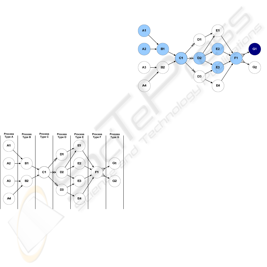
In Figure 1 there are seven process types (A, B,
…, G). Process type A has four instances. These
nodes have no predecessor which means that the
traced objects have been created in these nodes. The
objects are transferred forward in the graph. For
example, objects from Nodes A1 and A2 are
transferred to Node B1. Now objects are not
changed but object sets (product portions) of A1 and
A2 are unionized in B1. This also means that the
resources and emissions of A1 and A2 are
cumulated to the new set of objects. The objects
from B1 are transferred to the Node C1 where
products are classified and sent to one of the D
processes.
In the D processes objects are divided into
several objects. A double-headed arrow illustrates
this. For example a physical object is decomposed or
divided into parts. Then, parts may be classified and
sent to forthcoming processes. The E nodes receive
product portions consisting of these parts. In an E
process they are refined and sent to Node F1 which
is a shared process for all products. The products of
F1 are components for the G processes, i.e. in G1
and G2 objects are composed from the objects that
F1 yields. A shared start arrow illustrates this.
Figure 1: A sample traceability graph.
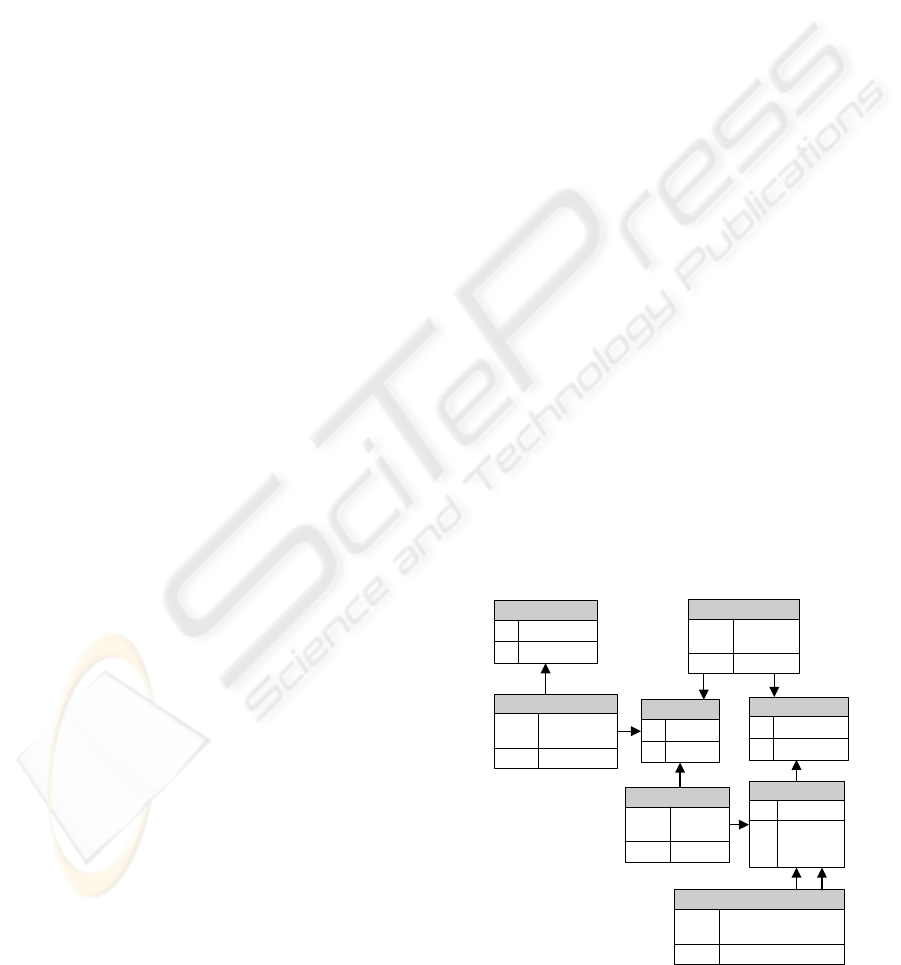
In a traceability graph it is possible to trace the
supply chain of an object, i.e. to find all the
preceding processes where the object at hand has
participated. This also means that all the information
related to those processes can be attached to the
object. Given the running example, let us assume
that we are interested in an object that belongs to
Node G1. Then, the processing history of the object
is a subgraph of the main graph. In Figure 2 the
colored nodes are processes in which the underlying
object, its part or a whole related to the parts has
participated. In the example, parts of the underlying
object have gone through F1, E2, E3 and D2,
whereas the larger objects consisting of the parts
have gone through C1, B1, A1 and A2. This
subgraph is also the supply chain of the underlying
object.
The traceability graph can also be used for
analyzing different aspects on processes. For
example a process type can be selected and we can
see how much some process causes the
environmental burden. Further, this analysis can be
done in a supply chain of one object or a set of
objects.
Figure 2: The supply chain of an objects belonging to
Node G1.
3.2 Data Management Primitives
Next, we introduce the properties of edges and nodes
of the traceability graph. For the reason of the
limited space the detailed and exact definitions of
the primitives associated with the traceability graph
are not given explicitly.
An object is the unit of tracing in a phase of the
related supply chain. This can be a single product or
a patch depending on the precision of tracing in the
underlying supply system.
A process node contains the identity of a
process, the set of product portions and the set of
attributes associated with the process. A product
portion involves the quantity of products, the
identifiers of objects and the ratio of the emissions
and resources compared with the total ones in the
process node. The ratio is calculated by an
application specific method. It can be based on the
portion of mass or used time of machines, for
example. Product portions of a process are viewed
through the end products of a process.
An attribute of a node determines information
associated with a process. In terms of input attributes
it can be described the resources of a process
whereas output attributes can be used for
determining the emissions of a process. Each
attribute has two values: one for the underlying
DATA MANAGEMENT FRAMEWORK FOR MONITORING AND ANALYZING THE ENVIRONMENTAL
PERFORMANCE
59
process and the other for containing the cumulated
values from the previous nodes. A cumulated value
is calculated based on the ratios of product portions
and quantity that is sifted from the previous nodes
via edges.
Via edges, products are sifted from a process to
another more precisely from a product portion to
another. An edge also determines the mapping of
objects between two processes. The mapping can be:
1. Equivalence: Objects from a start node of a
product portion are sifted to the related product
portion of the end node.
2. Subsetting: Only some objects are sifted to the
related product portion of the end node.
3. Supersetting: All the objects are sifted to the
related product portion of the end node but the
product portion of the end node contains similar
objects from another process node.
4. Division: Objects of a start node are divided
into smaller objects. If an object represents a
single product, this is portioned.
5. Composition: Products of the start nodes are
components for the end node.
In 1-3 the objects maintains their identities but in
4 and 5 the identities must be changed. In case 4 the
identity of a product is mapped with the identities of
parts that are produced from the product. In case 5
several objects are needed used for one composition,
i.e. the identities of components are mapped with the
identity of the related composition. It is worth noting
that a product of an end node may contain
components from several start nodes.
Through an edge the information of sifted
products from a node to another node is transferred
to an end node following the mapping of objects. An
edge involves those objects that are sifted from a
start node to the end node (only some products of a
product portion may be selected from other
processes). This part of the product portion of the
start node is called a sifted product portion. In
transferring products from a process to another, the
attributes must be re-calculated for corresponding to
the sifted product portion. This is based on the
ordinary and derived attributes. The derived
attribute is associated with an edge and it determines
the amount of an ordinary attribute that is related to
the sifted product portion.
4 IMPLEMENTING
TRACEABILITY GRAPH
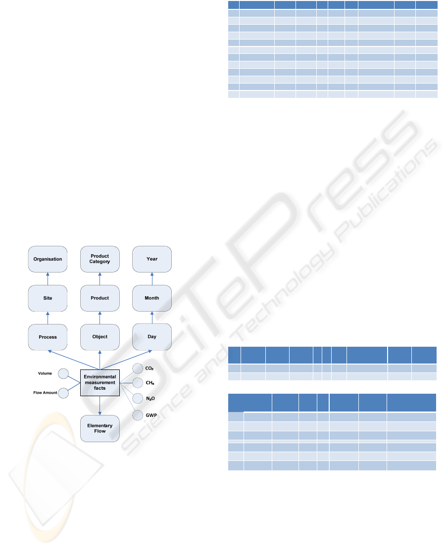
The traceability graph is mapped to the relational
database as presented in Figure 3. We selected the
relational database because the standard OLAP
(Online Analytic Processing) methods (Chaudhuri
and Dayal, 1997) are used to further analyze the
huge amount of data that is a result for tracing the
individual objects. In Figure 3 PK means primary
key and FK means foreign key.
The information of the traceability graph is
stored into eight relations:
• Node relation is used to store the identities of
process nodes.
• Attributes (e.g. raw materials, energy) are stored
into Attribute relation
• Product types are stored into Product relation.
• The relation NodeAttribute is used to store
the process (Node) specific attributes. For
example 〈Process#1, Electricity, 100 kWh〉
specifies the use of electricity of Process#1.
• The relation NodeProduct is used to store the
information about product portions of a specific
process (Node). The column Ratio is used to
allocate the environmental burden between the
portions of products and by-products. For
example 〈Process#1, Product#1, 0.6〉 specifies
that Product#1 is an end product of Process#1
and the related ratio is 0.6.
• The relation Object is used to store the object
specific information like physical code of the
object and its volume.
• The relation ObjectRelation is used to
store the object mapping when object identities
are changed. The column Transformation
function is used to calculate the cumulated
attribute values.
• The route of the objects through a supply chain
is realised by the Route relation. This
corresponds to the sifted product portion.
Figure 3: Database schema for the traceability graph.
Node
PK NodeKey
NodeAttribute
PK,FK1 NodeKey
PK,FK2 AttributeKey
AttributeValue
NodeProduct
PK,FK1 NodeKey
PK,FK2 ProductKey
Ratio
Attribute
PK AttributeKey
AttributeName
Product
PK ProductKey
ProductName
Route
PK,FK1 NodeKey
PK,FK2 ObjectKey
Time
Object
PK ObjectKey
ObjectCode
Volume
FK1 ProductKey
ObjectRelation
PK,FK1 ParentObjectKey
PK,FK2 ChildObjectKey
TransformationFunction
INNOV 2010 - International Multi-Conference on Innovative Developments in ICT
60
The relation model in Figure 3 can be easily
extended to include more product and supply chain
specific information. For example, we can
implement an organisational hierarchy by creating
Process, Site and Organisation relations
(Node→Process → Site→ Organisation).
This kind of extension enables analysis of
environmental data by using the hierarchy as a
dimension in multidimensional OLAP model.
5 TRACEABILITY CUBE
To be able to use the OLAP type operations for
analyzing the information of the traceability graph
we must combine the previous tables as a data cube.
In this work we will use the multidimensional data
model “MD” that is presented in (Torlone, 2003). In
Figure 4 the dimensions are presented as round-
cornered boxes, the facts are presented as boxes and
the measures as circles. The circles with drawn with
dashed line presents calculated measures.
Figure 4: Traceability cube scheme.
Figure 4 presents the traceability cube with some
example dimensions. The Process dimension can
be used to compare the environmental impact
between manufacturing sites and manufacturers. The
Object dimension is used to aggregating the
environmental data for different product groups. The
measure Flow Amount is the attribute amount for
an object. The measure Volume specifies the
volume of an object. In Table 1 some sample
instances over the traceability cube are presented.
The EPC column is the unique identity of an
object.
Table 1: A sample instance over the traceability cube.
The Flow Amount is used for calculating the
calculated measures – amount of emissions (e.g.
carbon dioxide, methane, nitrous oxides) and
amount of key environmental performance
indicators (see e.g. Lim and Park, 2009). The
emission amount is the amount of emissions caused
when using elementary flow (raw material or
energy) in some process. For example, carbon
dioxide emissions when using electricity from
Tampere electricity station in Finland were 194 g /
kWh in the year 2008. There are many
environmental databases that comprise life cycle
inventory data from different supply chain
processes. For example, the ELCD core database by
European Commission - DG Joint Research Centre -
Institute for Environment and Sustainability
comprises more than 300 process datasets (e.g. key
materials, energy carriers, transport, and waste
management).
Table 2: Emission and Impact Calculation.
↓
In Table 2 the emissions and impact category for
objects with code 2 and 4 are presented. Key
environmental performance indicators are calculated
based on the emissions. In this example we use the
global warming potential which is one commonly
used an environmental key performance indicator. It
is calculated based on carbon dioxide, methane,
nitrous oxide and several other emissions. The
measurement unit for the global warming potential is
kg of carbon dioxide equivalent which means that all
the other emissions are converted by using a
EPC Process Site Product Day Month Year
Flow Amount
Volume
1KilnDrying Mill#1 Timber 1 1 2010 Electricity 0,5kWh 0,30m³
2KilnDrying Mill#1 Timber 1 1 2010 Electricity 0,5kWh 0,35m³
3KilnDrying Mill#1 Timber 1 1 2010 Electricity 0,5kWh 0,33m³
1 Transporting Truck#1 Timber 2 1 2010 LorryTransport 100km 0,30m³
2 Transporting Truck#1 Timber 2 1 2010 LorryTransport 100km 0,35m³
3 Transporting Truck#1 Timber 2 1 2010 LorryTransport 100km 0,33m³
4KilnDrying Mill#1 Timber 1 1 2010 Electricity 0,53kWh 0,40m³
5KilnDrying Mill#1 Timber 1 1 2010 Electricity 0,53kWh 0,42m³
6KilnDrying Mill#1 Timber 1 1 2010 Electricity 0,53kWh 0,38m³
4 Transporting Train#1 Timber 2 1 2 010 RailTransport 20 0 km 0,40m³
5 Transporting Train#1 Timber 2 1 2 010 RailTransport 20 0 km 0,42m³
6 Transporting Train#1 Timber 2 1 2 010 RailTransport 20 0 km 0,38m³
EPC Process Site Product D M Year
Elementary
Flow
Flow
Amount
Volume
2 Transp. Truck#1 Timber 2 1 2010 LorryTransport 10 0 km 0,35m³
4 Transp. Truck#2 Timbe r 2 1 2010 RailTransport 200 km 0,40m³
EPC Emission Amount Unit
Impact
Category
Amount Unit
2CO₂ 19,9102 kg → GWP 19,9102 askgofCO₂eq.
2CH₄ 0,19636 g → GWP 0,004909 askgofCO₂eq.
2N₂O 0,15401 g → GWP 0,045895 askgofCO₂eq.
4CO₂ 22,1193 kg → GWP 22,1193 askgofCO₂eq.
4CH₄ 0,13933 g → GWP 0,003483 askgofCO₂eq.
4N₂O 8,63872 g → GWP 2,574338 askgofCO₂eq.
DATA MANAGEMENT FRAMEWORK FOR MONITORING AND ANALYZING THE ENVIRONMENTAL
PERFORMANCE
61
conversion factor. For example the conversion factor
of Methane is 25. Full list of emissions and factors
can be found from PAS 2050 (Carbon Trust 2008).
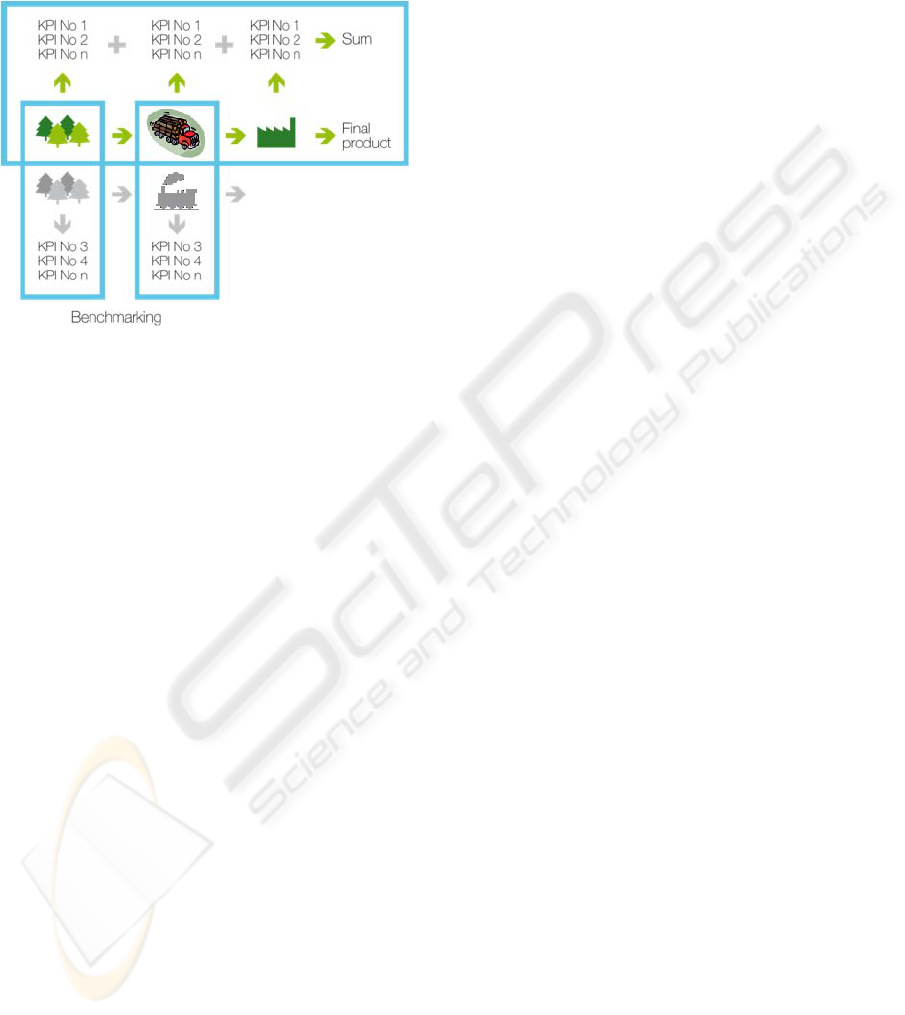
The analytics capabilities of the traceability cube
can be used for analyzing the environmental data.
Figure 5: Using the traceability cube.
For example, environmental data can be summed
up to create the total environmental impact for the
whole life cycle of the product. The data can also be
used for comparing the performance between
different manufacturers or manufacturing sites as
illustrated in Figure 5. The possibility to analyze the
supply chain on the process and item level allows
the end users to select a product which creates least
environmental burden. This creates pressure for the
manufacturers to improve the eco-efficiency of their
supply chains.
6 DISCUSSION
The precision of traceability of the resources and
emissions depends on the underlying data model and
ability how strictly physical products and their
components can be identified. Our model can be
applied to any granularity of tracing. For
applications, it is required physical identity
mechanism that can be mapped to their logical
counterparts in the database.
One option for marking the objects is Radio-
Frequency Identification (RFID) technology which
can be compared to the bar code identification: an
identification code is embedded to an object. In the
RFID technology the identification process does not
require a clear line of sight. The potential of the
RFID technology to monitor the carbon footprint of
products is demonstrated in (Dada et al., 2009, 2010;
Ilic et al., 2009).
7 CONCLUSIONS
We presented a model how emissions and resources
can be monitored from the data management
perspective. The model can be mapped to any
precision level of physical tracing. At the most
precise level, even a single physical object and its
components can be analyzed. This, of course,
demands that the related objects and their
components are identified and mapped to the
database. From the opposite perspective our model
also supports rough level analysis of products and
their histories. We showed how multidimensional
analysis can be applied for OLAP analysis based on
the traceability graph.
ACKNOWLEDGEMENTS
This work is supported by Academy of Finland
under grant #115480.
REFERENCES
Carbon Trust, 2008. Specification for the assessment of the
life cycle greenhouse gas emissions of goods and
services. PAS 2050:2008.
Chaudhuri, S. and Dayal, U., 1997. An Overview of Data
Warehousing and OLAP technology. ACM SIGMOD
Record 26(1), 65-74
Dada, A. Staake, T. Fleisch, E., 2009. The Potential of the
EPC Network to Monitor and Manage the Carbon
Footprint of Products: Carbon Accounting, Auto-ID
Labs White Paper WP-BIZAPP-047.
Dada, A. Rau, A. Konkel, M. Staake, T. Fleisch, E., 2010
The Potential of the EPC Network to Monitor and
Manage the Carbon Footprint of Products: Dynamic
Carbon Footprint Demonstrators. Auto-ID Labs
White Paper WP-BIZAPP-054.
Ilic, A. Staake, T. Fleisch, E., 2009 Using Sensor
Information to Reduce the Carbon Footprint of
Perishable Goods. IEEE Pervasive Computing. 8(1)
22-29.
Lim, S.-R. and Park, J. M., 2009. Environmental
indicators for communication of life cycle impact
assessment results and their applications. Journal of
Environmental Management 90 (19), 3305-3312.
Torlone, R. 2003. Conceptual Multidimensional Models.
In Multidimensional Databases: Problems and
Solutions. Idea Group Publishing, 69-90.
Usva, K. Hongisto, M. Saarinen, M. Katajajuuri, J.M.
Nissinen, A. Perrels, A. Nurmi, P. Kurppa, S. Koskela,
S., 2009. Towards certifies carbon footprints of
products – a road map for data production, VATT
Research Reports 143:2
INNOV 2010 - International Multi-Conference on Innovative Developments in ICT
62
