A GIBBS DISTRIBUTION THAT LEARNS FROM GA DYNAMICS

Manabu Kitagata and Jun-ichi Inoue

Complex Systems Engineering, Graduate School of Information Science and Technology

Hokkaido University, N14-W9, Kita-ku, Sapporo 060-0814, Japan

Keywords:

Genetic algorithms, Evolutionary optimization, Machine learning, Population dynamics, Thermodynamics,

Average-case performance, Spin glass model, Statistical physics.

Abstract:

A general procedure of average-case performance evaluation for population dynamics such as genetic algo-

rithms (GAs) is proposed and its validity is numerically examined. We introduce a learning algorithm of Gibbs

distributions from training sets which are gene conﬁgurations (strings) generated by GA in order to ﬁgure out

the statistical properties of GA from the view point of thermodynamics. The learning algorithm is constructed

by means of minimization of the Kullback-Leibler information between a parametric Gibbs distribution and

the empirical distribution of gene conﬁgurations. The formulation is applied to a solvable probabilistic model

having multi-valley energy landscapes, namely, the spin glass chain. By using computer simulations, we dis-

cuss the asymptotic behaviour of the effective temperature scheduling and the residual energy induced by the

GA dynamics.

1 INTRODUCTION

Genetic Algorithm (GA) (H.Holland, 1975) is a

heuristics to ﬁnd the best possible solution for com-

binatorial optimization problems and it is based on

several relevant operators such as selection, crossover

and mutation on the gene conﬁgurations (strings)

leading to transition from one state to the others. In

this paper, in order to ﬁgure out the statistical prop-

erties of GA from the view point of thermodynamics,

we introduce a learning algorithm of Gibbs distribu-

tions from training sets which are gene conﬁgurations

generated by GA. A procedure of average-case per-

formance evaluation for genetic algorithms is exam-

ined. The learning algorithm is constructed by means

of minimization of the Kullback-Leibler information

between a parametric Gibbs distribution and the em-

pirical distribution of gene conﬁgurations. The for-

mulation is applied to a solvable probabilistic model

having multi-valley energy landscapes, namely, the

spin glass chain (Li, 1981) in statistical physics. By

using computer simulations, we discuss the asymp-

totic behaviour of the effective temperature schedul-

ing and the residual energy induced by the GA dy-

namics.

2 GA AND SA

As we mentioned, in this paper,we consider the statis-

tical properties of GA from the view point of thermo-

dynamics. In simple GA, we deﬁne each gene conﬁg-

uration (member) by a string of binary variables with

length N, that is, s

s = (s

,··· ,s

),s

∈ {−1,+1},

and we attempt to make each conﬁguration in ensem-

ble with size M to the state which gives a minimum

of the energy function H(s

s), say, s

∗

D The problem

is systematically solved by GA if the system evolves

according to a Markovian process and the gene distri-

bution P

(t)

s) at time (generation)t might convergeas

(t)

s) →P

(∞)

s) and we have P

(∞)

s) = δ(s

s−s

∗

) =

∏

i=1

δ(s

−s

i∗

). On the other hand, one of the ef-

fective heuristics which is well-known as Simulated

Annealing (SA) (Kirkpatrick et al., 1983) is achieved

by inhomogeneous Markovian process. The process

is realized by Markov chain Monte Carlo method

(MCMC) which leads to an equilibrium Gibbs distri-

bution at temperature T = β

−1

(from now on, the β is

referred to as ‘inverse temperature’), namely,

(t)

s) =

−β

(t)

H(s

, Z =

∑

−β

(t)

H(s

. (1)

In SA, the temperature is scheduled very slowly in

time as β

(∞)

→ ∞ (T

(∞)

→ 0), and then, we can solve

295

Kitagata M. and Inoue J..

A GIBBS DISTRIBUTION THAT LEARNS FROM GA DYNAMICS.

DOI: 10.5220/0003047102950299

In Proceedings of the International Conference on Evolutionary Computation (ICEC-2010), pages 295-299

ISBN: 978-989-8425-31-7

 2010 SCITEPRESS (Science and Technology Publications, Lda.)

the problem as P

(∞)

s) = δ(s

s−s

∗

) =

∏

i=1

δ(s

−s

i∗

Therefore, both the GA and the SA share a concept

to make the distribution convergence to a single (or

several) delta-peak(s) at the solution(s). However, in

general, the Markovian (dynamical) process of GA is

very hard to treat mathematically due to the global

transition between the states by the crossoveror, espe-

cially, the mutation operator, whereas the SA causes

only local transitions between the states. From the

view point of EDA (Baluja, 1994), the dynamics of

GA should lead to an empirical distribution of states.

3 FORMULATION AND TOOLS

In this section, we explain our formulation and sev-

eral tools to evaluate the average-case performance of

GA through the effective temperature scheduling of

the Gibbs distribution that is trained from gene con-

ﬁgurations of simple GA.

3.1 Kullback-Leibler Information

We start our argument from the distance between an

empirical distribution from GA dynamics P

(t)

s) and

a Gibbs distribution P

(t)

s) at the effective tempera-

ture T = β

−1

. The distance is measured by the fol-

lowing Kullback-Leibler information (KL)

KL(P

) =

∑

s)log





(2)

where the summation with respect to all possible

gene conﬁgurations s

s = (s

,··· ,s

) is deﬁned by

∑

(···) ≡

∑

=±1

···

∑

=±1

(···). In this paper, we

represent each component of gene conﬁgurations by

= ±1 instead of s

= 0,1 because we choose the cost

function of spin glasses to be minimized as a bench-

mark test later on. The ‘spin’ here means a tiny mag-

net in atomic scale-length and s

= +1 stands for ‘up-

spin’ and vice versa. We should keep in mind that the

above distance is dependent on the inverse temper-

ature β. Thus, we obtain the following Boltzmann-

machine-type learning equation with respect to β as

dβ

= −

∂KL(P

(t)

)

∂β

∑

(t)

s) ·

∂P

(t)

s)/∂β

(t)

(3)

We naturally expect that the effective temperature

evolves so as to minimize the KL information for each

time step. When both distributions become identical

one in the limit of t → ∞, namely, P

(∞)

s) = P

(∞)

s),

we obtain

dβ

∑

(∞)

s) ·{∂P

(∞)

s)/∂β}/P

(∞)

= (∂/∂β)

∑

δ(s

s−s

∗

) = ∂α/∂β = 0 (4)

and the time evolution of inverse-temperature then

stops. We should notice that α ≡

∑

δ(s

s−s

∗

) is the

number of degeneracy at the lowest energy states.

3.2 Learning Equation for Spin Systems

Here we attempt to restrict ourselves to more particu-

lar problems, namely, we deal with a class of combi-

natorial optimization problems whose cost functions

are described by the energy function of Ising model.

We ﬁrst reformulate the equation (3) by means of

Ising spin systems having the energy function H(s

s) =

−

∑

. For the case of positive constant spin-

spin interaction J

= J > 0, ∀

i, j

, the lowest energy

state is apparently given by s

= +1, ∀

(all-up spins)

or s

= −1, ∀

(all-down spins). However, as we shall

see in the following sections, for the case of randomly

distributed J

(the ± sign is also random), the low-

est energy state is highly degenerated and it becomes

very hard to ﬁnd the state.

Substituting the corresponding Gibbs distribution

s) = exp[−βH(s

s)]/

∑

exp[−βH(s

s)] into equation

(3), the learning equation leads to

dβ

∑

−

∑

(

∑

)exp[β

∑

]

∑

exp[β

∑

]

(5)

where the second term appearing in the right hand

side of the above equation is internal energy of

the system described by the Hamiltonian H(s

s) =

−

∑

at temperature T = β

−1

, whereas the ﬁrst

term is the energy H(s

s) averaged over the empirical

distribution P

s) of GA. Then, we immediately ﬁnd

that the condition

∑

s)(

∑

) =

∑

s)(

∑

)

∑

(

∑

)exp[β

∑

]

∑

exp[β

∑

]

(6)

yields dβ/dt = 0 for P

s) = P

s).

In general, it is very hard to calculate the internal

energy of the spin system

U({J}: β) ≡ −

∑

(

∑

)exp[β

∑

]

∑

exp[β

∑

]

(7)

ICEC 2010 - International Conference on Evolutionary Computation

296

because 2

sums for all possible conﬁgurations in

∑

(···) are needed to evaluate the E({ J} : β), where

we deﬁned a set of interactions by {J} ≡ {J

|i, j =

1,··· ,N}. To overcome this difﬁculty, we usually use

the so-called Markov chain Monte Carlo (MCMC)

method to calculate the expectation (7) by important

sampling from the Gibbs distribution at temperature

T = β

−1

On the other hand, the ﬁrst term appearing in the

right hand side of (5), we evaluate the expectation by

making use of

({J}) ≡ −

∑

= − lim

L→∞

∑

l=1

∑

(t,l)s

(t,l)

(8)

where s

(t,l) is the l-th sampling point at time t from

the empirical distribution of GA. Namely, we shall

replace the expectation of the cost function H(s

s) =

−

∑

over the distribution P

s) by sampling

from the empirical distribution of GA.

By a simple transformation β → T

−1

in equation

(5), we obtain the Boltzmann-machine-type learning

equation with respect to effective temperature T as

follows.

= −T



U({J}: T

−1

) −U

({J})



(9)

From this learning equation, we ﬁnd that time-

evolution of effective temperature depends on the dif-

ference between the expectations of the cost function

over the Gibbs distribution at temperature T and the

empirical distribution of GA.

3.3 Average-case Performance

We should evaluate the ‘average-case performance’of

the learning equation which is independent of the re-

alization of ‘problem’ {J}. Namely, one should eval-

uate the ‘data-averaged’ learning equation

= −T



{J}



U({J}: T

−1

)



−E

{J}

({J}))



(10)

to discuss the average-case performance, where

we deﬁned the average E

{J}

(···) by E

{J}

(···) ≡

∏

(···)P(J

). We should keep in mind that

in this paper we deal with the problem in which

each interaction J

has no correlation with the oth-

ers, namely, E

{J}

) = J

i,k

j,l

where we de-

ﬁned J

as a variance of P(J

) and δ

x,y

stands for a

Kronecker’s delta.

4 MATHEMATICALLY

TRACTABLE MODEL

In this section, we introduce a spin glass model which

will be used as a benchmark cost function to be mini-

mized by GA. The model is called as spin glass chain.

It is one-dimensional spin glass model having only

nearest neighboring interactionsD It is possible for us

to investigate the temperature dependence of internal

energy and moreover, one can obtain the lowest en-

ergy exactly. The energy function (Hamiltonian in the

literature of statistical physics) is given by

H = −

∑

i=1

i+1

, J

= N (0, 1) (11)

where J

stands for the interaction between spins s

and s

i+1

. N (a, b) denotes a normal Gaussian distri-

bution with mean a variance bD We plot the typical

-2

-1.5

-1

-0.5

0.5

1.5

0 200 400 600 800 1000

H/N

N = 10

-0.8

-0.7

-0.6

-0.5

-0.4

-0.3

-0.2

-0.1

0 0.5 1 1.5 2 2.5 3 3.5 4 4.5 5

Theory

N = 3000, MCS = 20000

-5.5

-5

-4.5

-4

-3.5

-3

-2.5

-2

-1.5

-1

-0.5

0 1 2 3 4 5

min

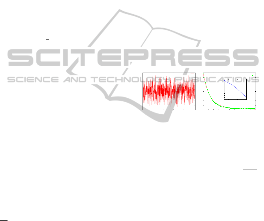
Figure 1: Typical energy landscape H(s

s) = −

∑

i+1

with P(J

) = N (0,1), E(J

) = δ

i, j

of the spin glass chain.

The number of spins is N = 10. It should be noted that

the horizontal axis S denotes the label of states, that is,

S = 1, 2,··· ,2

(= 1028). For instance, S = 1 stands for a

state, say, s

s(S = 1) = (+1,+1,··· , +1) and S = 2

denotes

s(S = 2

) = (−1, −1,··· ,−1). The right panel stands for

internal energy of spin glass chain as a function of temper-

ature. The solid line is exact result U = −β

∞

−∞

cosh

βx

whereas the dots denote the internal energy calculated by

the MCMC for N = 3000. The error-bars are calculated

by 10-independent runs for different choice of the {J} ≡

|i = 1,··· ,N}. The inset indicates the U

min

as a function

of J

. We set J = 1.

energy landscape in Figure 1 (left). From this ﬁgure,

we ﬁnd that the structure of the energy surface is com-

plicated and it seems to be difﬁcult for us to ﬁnd the

lowest energy state.

However, we should notice that in (11) s

takes ±1

and the product s

i+1

also has a value ±1. Hence, we

introduce the new variable τ

which is deﬁned by τ

i+1

, then τ

takes τ

∈ {1, −1}. Therefore, in order

to minimize H(τ

τ) = −

∑

, we should determine

= sgn(J

) for each i and then, we have the lowest

energy as U

min

= −

∑

sgn(J

) = −

∑

|. Namely,

when J

obeys a Gaussian with mean J

and variance

, the lowest energy for a single spin is obtained in

A GIBBS DISTRIBUTION THAT LEARNS FROM GA DYNAMICS

297

the thermodynamic limit N → ∞ as

lim

N→∞

min

= E

{J}

(|J

|) =

∞

−∞

√

2πJ

−

−J

)

= −J

−J

−

where E

{J}

(···) here stands for the average over the

conﬁguration {J} ≡ (J

,··· ,J

Thus, for the choice of (J

,J) = (1, 0), namely, in

the limit of the ferromagnetic Ising model, we have

the lowest energy as U

min

/N = −1 (all spins align in

the same direction), On the other hand, for the choice

of (J

,J) = (0,1), we have U

min

= −

2/π. These

facts mean that the lowest energy changes according

to the value of ratio J

/J.

We next consider the case of ﬁnite effective tem-

perature, namely, β < ∞. For this case, internal en-

ergy per spin is explicitly given by lim

N→∞

hHi

/N =

{J}

(hHi

) = −(∂/∂β)log

∑

with h···i

≡

∑

exp[β

∑

]/Z

where we deﬁned

∑

(···) ≡

∑

=±1

···

∑

=±1

(···) and the partition function

∑

is now calculated as {2cosh(βJ

)}

Hence, we have the average free energy density de-

ﬁned by f = lim

N→∞

(logZ/N) = N

−1

{J}

(logZ) is

evaluated as follows.

f =

∞

−∞

Dxlog2coshβ(J

+ Jx) (12)

where we deﬁned Dx ≡ dxe

−x

√

2π. From the

above result, we immediately obtain the internal en-

ergy per spin U = −∂f/∂β by

U = −β

∞

−∞

cosh

βx

. (13)

for the case of (J

,J) = (0, 1). In Figure 1 (right), we

show the U as a function of T. From the arguments

we provided above, we have the following learning

equation (14) for the spin glass chain whose Hamilto-

nian is given by (11) is now rewritten as

= T

lim

L→∞

∑

l=1

∑

(t,l)s

i+1

(t,l)

− T

∞

−∞

cosh

−1

. (14)

5 RESULTS

The results are summed up below. We show the time-

evolution of effective temperature (14) and the resid-

ual energy for the case of spin glass chain with pa-

rameter sets: σ = 2 (The number of members in selec-

tion of tournament -type at each generation), p

= 0.1

(The rate for a single point crossover), p

= 0.001

(The mutation rate) in Figure 2. From this ﬁgure,

we ﬁnd that the asymptotic behaviour of the effec-

tive temperature follows a power-law. This schedule

is faster than the effective temperature scheduling for

the optimal simulated annealing ∼ 1/log(1+t) (Ge-

man and Geman, 1984), however, slower than the ex-

ponential decreasing. Thus, here we deﬁne the resid-

ual energy and its time-dependence as the difference

between the lowest energy and current energy ob-

tained by the GA dynamics. We ﬁnd that the residual

energy which is deﬁned by

ε ≡ H(s

s) −min

H(s

s) (15)

also asymptotically goes to zero and it follows a

power-law in the scaling regime t ≫ 1.

0 200 400 600 800 1000 1200 1400

0.5

1.5

2.5

3.5

0 1 2 3 4 5 6 7

log(T)

log(t)

0.2

0.3

0.4

0.5

0.6

0.7

0.8

0 200 400 600 800 1000 1200 1400

-1.4

-1.2

-1

-0.8

-0.6

-0.4

-0.2

0 1 2 3 4 5 6 7

log(ε)

log(t)

Figure 2: Time evolution of the effective temperature (up-

per panel) and the residual energy deﬁned by (15) (lower

panel) for the case of spin glass chain. We used a simple

GA having σ = 2, p

= 0.1, p

= 0.001. We set the number

of spins N = 2000 and population M = 100, respectively.

The inset stands for the asymptotic behaviour.

6 CONCLUDING REMARKS

We introduced a learning algorithm of Gibbs dis-

tributions from training sets which are gene strings

generated by GA to ﬁgure out the statistical prop-

erties of GA from the view point of thermodynam-

ics. A procedure of average-case performance eval-

uation for genetic algorithms was numerically ex-

amined. The formulation was applied to a solvable

probabilistic model having multi-valley energy land-

scapes, namely, the spin glass chain. By using com-

puter simulations, we discussed the asymptotic be-

haviour of the effective temperature scheduling and

the residual energy induced by the GA dynamics.

REFERENCES

Baluja, S. (1994). Population-based incremental learning:

A method for integrating genetic search based func-

tion optimization and competitive learning. Technical

Report, School of Computer Science, Carnegie Mellon

University, CMU-CS-94:163.

ICEC 2010 - International Conference on Evolutionary Computation

298

Geman, S. and Geman, D. (1984). Stochastic relaxation,

gibbs distributions, and the bayesian restoration of im-

ages. IEEE Trans. on Pattern Analysis and Machine

Intelligence, PAMI-6:721–741.

H.Holland, J. (1975). Adaptation in natural and artiﬁcial

systems. The University of Michigan Press.

Kirkpatrick, S., D.Galatt, C., and P.Vecchi, M. (1983). Op-

timization by simulated annealing. Science, 220:671–

680.

Li, T. (1981). Structure of metastable states in a random

ising chain. Physical Review B, 24:6579–6587.

A GIBBS DISTRIBUTION THAT LEARNS FROM GA DYNAMICS

299