
OFP CLASS: AN ALGORITHM TO GENERATE OPTIMIZED
FUZZY PARTITIONS TO CLASSIFICATION
Jos´e M. Cadenas, M. del Carmen Garrido, Raquel Mart´ınez and Enrique Mu˜noz
Dpto. de Ingenier´ıa de la Informaci´on y las Comunicaciones, Facultad de Inform´atica
Universidad de Murcia, Murcia, Spain
Keywords:
Fuzzy discretization, Fuzzy set, Genetic algorithm, Fuzzy decision tree.
Abstract:
The discretization of values is a important role in data mining and knowledge discovery. The representation
of information through intervals is more concise and easier to understand at certain levels of knowledge than
the representation by mean continuous values. In this paper, we propose a method for discretizing continuous
attributes by means a series of fuzzy sets which constitute a fuzzy partition of this attribute’s domain. We
present an algorithm, which carries out a fuzzy discretization of continuous attributes in two stages. In the first
stage a fuzzy decision tree is used and the genetic algorithm is used in the second stage. In this second stage
the cardinality of the partition is defined. After defining the fuzzy partitions these are evaluated by a fuzzy
decision tree which is also detailed in this study.
1 INTRODUCTION
The selection, processing and data cleaning is one of
the phases making up the process of knowledge dis-
covery. This phase can be very important for some
algorithms of classification, because the data must
be preprocessed so that the algorithm can work with
them. A possible change in the data may be the
discretization of continuous values. The discretiza-
tion continuous attributes can be carried out through
crisp partitions or fuzzy partitions. Crisp partitions
use classical logic, where each attribute is split into
several intervals, whereas fuzzy partitions use fuzzy
logic. On the one hand, we can find techniques to dis-
cretize continuous attributes into crisp intervals, (Liu
et al., 2002), (Catlett, 1991), in which a domain value
can only belong to a partition or interval. On the
other hand we find methods to discretize continuous
attributes into fuzzy intervals (Li, 2009), (Li et al.,
2009), in this case, a domain value can belong to more
than one element of the fuzzy partition.
In this study we present the OFP
CLASS Algo-
rithm to carry out a fuzzy discretization of continuous
attributes, which is divided in two stages. In the first
stage, we carry out a search of split points for each
continuous attribute. In the second stage, based on
these split points, we use a genetic algorithm which
optimizes the fuzzy sets formed from the split points.
Having designed the fuzzy sets that make up the fuzzy
partition of each continuous attribute, they are evalu-
ated with a classifier constituted by a fuzzy decision
tree.
The structure of this study is as follows. In Section
2, we are going to present a taxonomy of discretiza-
tion methods, as well a review various discretization
methods. Then, in Section 3, we are going to present
the OFP CLASS Algorithm, which is based on a deci-
sion tree and a genetic algorithm, as our proposal for
the problem of fuzzy discretization applied to clas-
sification. Next, in Section 4, we will show various
experimental results which evaluate our proposal in
comparison with previously existing ones and where
the results have been statistically validated. Finally, in
Section 5, we will show the conclusions of this study.
2 DISCRETIZATION METHODS
The classification is one of the most important topics
in data mining area. There are many different classi-
fication methods which work with continuous values
and/or discrete values. However, not all classification
algorithms can work with continuous data, hence dis-
cretization techniques are needed to these algorithms.
Although, there are algorithms which work with dis-
crete data by the fact that they can improve results in
classification tasks.
5
M. Cadenas J., del Carmen Garrido M., Martínez R. and Muñoz E..
OFP_CLASS: AN ALGORITHM TO GENERATE OPTIMIZED FUZZY PARTITIONS TO CLASSIFICATION.
DOI: 10.5220/0003052700050013
In Proceedings of the International Conference on Fuzzy Computation and 2nd International Conference on Neural Computation (ICFC-2010), pages
5-13
ISBN: 978-989-8425-32-4
Copyright
c
2010 SCITEPRESS (Science and Technology Publications, Lda.)

When a discretization process is to be developed,
four iterative stages must be carried out, (Liu et al.,
2002):
1. The values in the database of the continuous at-
tributes to be discretized are ordered.
2. The best split point for partitioning attribute do-
mains in the case of top-down methods is found,
or the best combination of adjacent partitions for
bottom-up methods is found.
3. If the method is top-down, once the best split
point is found, the domain of each attribute is di-
vided into two partitions, and when the method is
bottom-up, both partitions are merged.
4. Finally, we check whether the stopping criterion
is fulfilled, and if so the process is terminated.
In this general discretization process we have dif-
ferentiated between top-down and bottom-up algo-
rithms. However, there are more complex taxonomies
for the different methods of discretization such as that
presented in (Liu et al., 2002) and which are shown
here:
• Supervised or non-supervised. Non-supervised
methods are those based solely on continuous at-
tribute value in order to carry out discretization,
whereas supervised ones use class value to dis-
cretize continuous attributes, so that they are more
or less uniform with regard to class value.
• Static or dynamic. In both types of methods it
is necessary to define a maximum number of in-
tervals and they differ in that static methods seek
to divide each attribute in partitions sequentially,
whereas dynamic ones discretize domains by di-
viding all the attributes into intervals simultane-
ously.
• Local or Global. Local methods of discretization
are those which use algorithms such as C4.5 or its
successor C5.0, (Quilan, 1993), and they are only
applied to specific regions in the database. On the
other hand, global methods are based on the whole
database to carry out discretization.
• Top-down or Bottom-up. Top-down methods
begin with an empty list of split points and add
them as the discretization process finds intervals.
On the other hand, bottom-up methods begin with
a list full of split points and eliminate points dur-
ing the discretization process.
• Direct or Incremental. Direct methods divide
the dataset directly into k intervals. Thereforethey
need an external input determined by the user to
indicate the number of intervals. Incrememental
methods begin with a simple discretization and
undergo an improvement process. For this rea-
son they need a criterion to indicate when to stop
discretizing.
In addition to the taxonomy exposed, from an-
other viewpoint we consider discretization methods
can also be classified according to the type of parti-
tions constructed, crisp or fuzzy partitions.
Thus, in the literature we find some algorithms
that generate crisp partitions. Among these, in (Holte,
1993) describes a method that performs crisp intervals
taken as a measure the amplitude or frequency, which
need to fix a k number of intervals. Also, (Holte,
1993) describes other method, called R1, which needs
to have a fixed number of k intervals, but in this case,
the measure which used is the class label. Another
method that constructs crisp partitions, D2, is de-
scribed in (Catlett, 1991), where the measure used is
entropy.
On the other hand, we find methods which dis-
cretize continuous values in fuzzy partitions, in this
case, these methods use decision trees, clustering al-
gorithms, genetic algorithms, etc. So, in (Kbir et al.,
2000) a hierarchical fuzzy partition based on 2
|A|
-tree
decomposition is carried out, where |A| is the num-
ber of attributes in the system. This decomposition
is controlled by the degree of certainty of the rules
generated for each fuzzy subspace and the deeper hi-
erarchical level allowed. The fuzzy partitions formed
for each domain are symmetric and triangular. Fur-
thermore, one of the most widely used algorithms for
fuzzy clustering is fuzzy c-means (FCM) (Bezdek,
1981). The algorithm assigns a set of examples, char-
acterized by their respective attributes, to a set number
of classes or clusters. Some methods developed for
fuzzy partitioning start from the FCM algorithm and
add some extension or heuristic to carry out an opti-
mization in the partitions. We can find some examples
in (Li, 2009), (Li et al., 2009). Also, a method that
constructs fuzzy partition using a genetic algorithm
is proposed in (Piero et al., 2003), where fuzzy par-
titions are obtained through beta and triangular func-
tions. The construction process of fuzzy partitions is
divided into two stages. In the first stage, fuzzy par-
titions with beta (Cox et al., 1998) or triangular func-
tions are constructed; and in the second stage these
partitions are adjusted with a genetic algorithm.
ICFC 2010 - International Conference on Fuzzy Computation
6

3 OFP CLASS: AN ALGORITHM
TO GENERATE OPTIMIZED
FUZZY PARTITIONS TO
CLASSIFICATION
In this section, the OFP CLASS Algorithm we pro-
pose for discretizing continuous attributes by means
of fuzzy partitions is presented and it is may be cat-
alogued as supervised and local. The OFP CLASS
Algorithm is made up of two stage. In the first stage,
crisp intervals are defined for each attribute. In the
second stage, these intervals obtained are used to form
an optimal fuzzy partition for classification using a
genetic algorithm, but not all the crisp intervals ob-
tained are used, because the genetic algorithm is who
determines which intervals are the best. The partition
obtained for each attribute guarantees the:
• Completeness (no point in the domain is outside
the fuzzy partition), and
• Strong fuzzy partition (it verifies that ∀x ∈ Ω
i
,
∑
F
i
f=1
µ
B
f
(x) = 1, where B
1
, .., B
F
i
are the F
i
fuzzy
sets for the partition corresponding to the i contin-
uous attribute with Ω
i
domain).
The domain of each i continuous attribute is parti-
tioned in trapezoidal fuzzy sets, B
1
, B
2
.., B
F
i
, so that:
µ
B
1
(x) =
1 b
11
≤ x ≤ b
12
(b
13
−x)
(b
13
−b
12
)
b
12
≤ x ≤ b
13
0 b
13
≤ x
;
µ
B
2
(x) =
0 x ≤ b
12
(x−b
12
)
(b
13
−b
12
)
b
12
≤ x ≤ b
13
1 b
13
≤ x ≤ b
23
(b
24
−x)
(b
24
−b
23
)
b
23
≤ x ≤ b
24
0 b
24
≤ x
;
··· ;
µ
B
F
i
(x) =
0 x ≤ b
(F
i
−1)3
(x−b
(F
i
−1)3
)
(b
(F
i
−1)4
−b
(F
i
−1)3
)
b
(F
i
−1)3
≤ x ≤ b
(F
i
−1)4
1 b
F
i
3
≤ x
Before going into a detailed description of
OFP CLASS Algorithm, we are going to introduce
the nomenclature we are going to use throughout the
section and then we will present the fuzzy decision
tree to be used in the evaluation of the fuzzy parti-
tions generated and which, with some modification,
is used in the first stage of OFP CLASS Algorithm.
3.1 Nomenclature and Basic
Expressions
• N: Node which is being explored at anygiven mo-
ment.
• C: Set of classes or possible values of the decision
attribute. |C| denotes the C set cardinal.
• E: Set of examples from the dataset.|E| denotes
the number of examples from the dataset.
• e
j
: j-th example from the dataset.
• A: Set of attributes which describe an example
from the dataset. |A| denotes the number of at-
tributes that describe an example.
• G
N
i
: information gain when node N is divided by
attribute i.
G
N
i
= I
N
− I
S
N
V
i
(1)
where:
– I
N
: Standard information associated with node
N. This information is calculated as follows:
1. For each class k = 1, ..., |C|, the value P
N
k
,
which is the number of examples in node N
belonging to class k is calculated:
P
N
k
=
|E|
∑
j=1
χ
N
(e
j
) · µ
k
(e
j
) (2)
where:
· χ
N
(e
j
) the degree of belonging of example
e
j
to node N.
· µ
k
(e
j
) is the degree of belonging of example
e
j
to class k.
2. P
N
, which is the total number of examples in
node N, is calculated.
P
N
=
|C|
∑
k=1
P
N
k
3. Standard information is calculated as:
I
N
= −
|C|
∑
k=1
P
N
k
P
N
· log
P
N
k
P
N
– I
S
N
V
i
is the product of three factors and repre-
sents standard information obtained by divid-
ing node N using attribute i adjusted to the ex-
istence of missing values in this attribute.
I
S
N
V
i
= I
S
N
V
i
1
· I
S
N
V
i
2
· I
S
N
V
i
3
where:
OFP_CLASS: AN ALGORITHM TO GENERATE OPTIMIZED FUZZY PARTITIONS TO CLASSIFICATION
7

∗ I
S
N
V
i
1
= 1 -
P
N
m
i
P
N
, where P
N
m
i
is the weight of
the examples in node N with missing value in
attribute i.
∗ I
S
N
V
i
2
=
1
∑
H
i
h=1
P
N
h
, H
i
being the number of descen-
dants associated with node N when we divide
this node by attribute i and P
N
h
the weight of
the examples associated with each one of the
descendants.
∗ I
S
N
V
i
3
=
∑
H
i
h=1
P
N
h
·I
N
h
, I
N
h
being the standard in-
formation of each descendant h of node N.
3.2 A Fuzzy Decision Tree
In this section, we describe the fuzzy decision tree
that we will use as a classifier to evaluate fuzzy par-
titions generated and whose basic algorithm will be
modified for the first stage of the OFP CLASS Algo-
rithm, as we will see later.
The set of examples E out of which the tree is
constructed is made up of examples described by at-
tributes which may be nominal, discrete and continu-
ous, and where there will be at least one nominal or
discrete attribute which will act as a class attribute.
The algorithm by means of which we construct the
fuzzy decision tree is based on the ID3 algorithm,
where all the continuous attributes have been dis-
cretized by means of a series of fuzzy sets.
An initial value equal to 1 (χ
root
(e
j
) = 1) is as-
signed to each example e
j
used in the tree learning,
indicating that initially the example is only in the root
node of the tree. This value will continue to be 1 as
long as the example e
j
does not belong to more than
one node during the tree construction process. In a
classical tree, an example can only belong to one node
at each moment, so its initial value (if it exists) is not
modified throughout the construction process. In the
case of a fuzzy tree, this value is modified in two sit-
uations:
• When the example e
j
has a missing value in an
attribute i which is used as a test in a node N.
In this case, the example descends to each child
node N
h
, h = 1, ...,H
i
with a modified value as
χ
N
h
(e
j
) = χ
N
(e
j
) ·
1
H
i
.
• According to e
j
’s degree of belonging to differ-
ent fuzzy partition sets when the test of a node
N is based on attribute i which is continuous. In
this case, the example descends to those child
nodes to which the example belongs with a de-
gree greater than 0 (µ
B
f
(e
j
) > 0; f = 1, ..., F
i
).
Because of the characteristics of the partitions
we use, the example may descend to two child
nodes at most. In this case, χ
N
h
(e
j
) = χ
N
(e
j
) ·
µ
B
f
(e
j
); ∀ f| µ
B
f
(e
j
) > 0; h = f.
We can say that the χ
N
(e
j
) value indicates the de-
gree with which the example fulfills the conditions
that lead to node N on the tree.
The stopping condition is defined by the first con-
dition reached out of the following: (a) pure node, (b)
there aren’t any more attributes to select, (c) reaching
the minimum number of examples allowed in a node.
Having constructed the fuzzy tree, we use it to infer
an unknown class of a new example:
Given the example e to be classified with the ini-
tial value χ
root
(e) = 1, go through the tree from the
root node. After obtain the leaf set reached by e. For
each leaf reached by e, calculate the support for each
class. The support for a class on a given leaf N is ob-
tained according to the expression (2). Finally, obtain
the tree’s decision, c, from the information provided
by the leaf set reached and the value χ with which
example e activates each one of the leaves reached.
In the following sections we describe the stages
which comprise the Algorithm of discretization
OFP CLASS.
3.3 First Stage: Looking for Crisp
Intervals
In this stage, a fuzzy decision tree is constructed
whose basic process is that described in subsection
3.2, except that now a procedure based on priority
tails is added and there are continuous attributes that
have not been discretized. The discretization of these
attributes is precisely the aim of this first stage.
To deal with non-discretized continuous at-
tributes, the algorithm follows the basic process in
C4.5. The thresholds selected in each node of the tree
for these attributes will be the split points that delimit
the intervals. Thus, the algorithm that constitutes this
first stage is based on a fuzzy decision tree that allows
nominal attributes, continuous attributes discretized
by means of a fuzzy partition, non-discretized con-
tinuous attributes, and furthermore it allows the exis-
tence of missing values in all of them. Algorithm 1
describes the whole process.
3.4 Second Stage: Constructing and
Optimizing Fuzzy Partitions
Genetic algorithms are very powerful and very robust,
as in most cases they can successfully deal with an in-
finity of problems from very diverse areas. These al-
gorithms are normally used in problems without spe-
cialized techniques or even in those problems where
ICFC 2010 - International Conference on Fuzzy Computation
8

Algorithm 1: Search of crisp intervals
SearchCrispIntervals(in : E, Fuzzy Partition;
out : Split points)
begin
1. Start at the root node, which is placed in the ini-
tially empty priority tail. Initially, the root node
is found in the set of examples E with an initial
weight of 1. The tail is a priority tail, ordered
from higher to lower according to the total weight
of the examples of nodes that form the tail. Thus
the domain is guaranteed to partition according to
the most relevant attributes.
2. Extract the first node from the priority tail.
3. Select the best attribute to divide this node using
information gain expressed in (1) as the criterion.
We can find two cases. The first case is where
the attribute with the highest information gain is
already discretized, either because it is nominal,
or else because it had already been discretized
earlier by the Fuzzy Partition. The second case
arises when the attribute is continuous and non-
discretized, in which case it is necessary to obtain
the corresponding split points.
(a) If the attribute is already discretized, node N is
expanded into as many children as possible val-
ues the selected attribute may have. In this case,
the tree’s behaviour is similar to that described
in the Subsection 3.2.
(b) If the continuous attribute is not previously dis-
cretized, its possible descendants are obtained.
To do this, as in C4.5, the examples are ordered
according to the value of the attribute in ques-
tion and the intermediate value between the
value of the attribute for example e
j
and for ex-
ample e
j+1
is obtained. The value obtained will
be that which provides two descendants for the
node and to which the criterion of information
gain is applied. This is repeated for each pair
of consecutive values of the attribute, search-
ing for the value that yields the greatest infor-
mation gain. The value that yields the greatest
information gain will be the one used to divide
the node and will be considered as a split point
for the discretization of this attribute.
4. Having selected the attribute to expand node N,
all the descendants generated are introduced in the
tail according to the established order.
5. Go back to step two to continue constructing the
tree until there are not nodes in the priority tail or
until another stopping condition occurs, such as
reaching nodes with a minimum number of exam-
ples allowed by the algorithm.
end
a technique does exist, but is combined with a genetic
algorithm to obtain hybrid algorithms that improvere-
sults (Cox, 2005).
In this second stage of the OFP CLASS Algo-
rithm, we are going to use a genetic algorithm to
obtain the fuzzy sets that make up the partitioning
of continuous attributes of the problem. Given the
F
i
− 1 split points of attribute i obtained in the prior
stage, we can define a maximum of F
i
fuzzy sets
that perform up the partition of i. The definition
of the different elements that make up this genetic
algorithm is as follows:
Encoding. An individual will consist of two array
v
1
and v
2
. The array v
1
has a real coding and its
size will be the sum of the number of split points that
the fuzzy tree will have provided for each attribute in
the first stage. Each gene in array v
1
represents the
quantity to be added to and subtracted from each at-
tribute’s split point to form the partition fuzzy. On
the other hand, the array v
2
has a binary coding and
its size is the same that the array v
1
. Each gene in
array v
2
indicates whether the corresponding gene or
split point of v
1
is active or not. The array v
2
will
change the domain of each gene in array v
1
. The do-
main of each gene in array v
1
is an interval defined
by [0, min(
p
r
−p
r−1
2
,
p
r+1
−p
r
2
)] where p
r
is the r-th split
point of attribute i represented by this gene except in
the first (p
1
) and last (p
u
) split point of each attribute
whose domains are, respectively: [0, min(p
1
,
p
2
−p
1
2
]
and [0, min(
p
u
−p
u−1
2
, 1− p
u
].
When F
i
= 2, the domain of the single split point
is defined by [0, min(p
1
, 1− p
1
]. The population size
will be 100 individuals.
Initialization. First the array v
2
in each individual
is randomly initialized, provided that the genes of
the array are not all zero value, since all the split
points would be deactivated and attributes would
not be discretized. Once initialized the array v
2
,
the domain of each gene in array v
1
is calculated,
considering what points are active and which not.
After calculating the domain of each gene of the
array v
1
, each gene is randomly initialized generating
a value within its domain.
Fitness Function. The fitness function of each in-
dividual is defined according to the information gain
defined in (Au et al., 2006). Algorithm 2 implements
the fitness function, where:
• µ
if
is the belonging function corresponding to
fuzzy set f of attribute i.
• E
k
is the subset of examples of E belonging to
class k.
OFP_CLASS: AN ALGORITHM TO GENERATE OPTIMIZED FUZZY PARTITIONS TO CLASSIFICATION
9

This fitness function, based on the information
gain, indicates how dependent the attributes are
with regard to class, i.e., how discriminatory each
attribute’s partitions are. If the fitness we obtain
for each individual is close to zero, it indicates
that the attributes are totally independent of the
classes, which means that the fuzzy sets obtained
do not discriminate classes. On the other hand, as
the fitness value moves further away from zero,
it indicates that the partitions obtained are more
than acceptable and may discriminate classes
with good accuracy.
Algorithm 2: Fitness Function.
Fitness(in : E, out : ValueFitness)
begin
1. For each attribute i = 1, ...,|A|:
1.1 For each set f = 1, ..., F
i
of attribute i
For each class k = 1, ..., |C| calculate the probabil-
ity
P
ifk
=
Σ
eεE
k
µ
if
(e)
Σ
eεE
µ
if
(e)
1.2 For each class k = 1, ..., |C| calculate the probabil-
ity
P
ik
= Σ
F
i
f=1
P
ifk
1.3 For each f = 1, ..., F
i
calculate the probability
P
if
= Σ
|C|
k=1
P
ifk
1.4 For each f = 1, ...,F
i
calculate the information
gain of attribute i and set f
I
if
= Σ
|C|
k=1
P
ifk
· log
2
P
ifk
P
ik
· P
if
1.5 For each f = 1, ..., F
i
calculate the entropy
H
if
= −Σ
|C|
k=1
P
ifk
· log
2
P
ifk
1.6 Calculate the I and H total of attribute i
I
i
=
F
i
∑
f=1
I
if
and H
i
=
F
i
∑
f=1
H
if
2. Calculate the fitness as :
ValueFitness =
∑
|A|
i=1
I
i
∑
|A|
i=1
H
i
end
Selection. Individual selection is by means of
tournament, taking subsets with size 2.
Crossing. The crossing operator is applied with a
probability of 0.3, crossing two individuals through a
single point, which may be any one of the positions
on the vector. Not all crossings are valid, since one of
the restrictions imposed on an individual is that the
array v
2
should not has all its genes to zero. When
crossing two individuals and this situation occurs,
the crossing is invalid, and individuals remain in
the population without interbreeding. If instead the
crossing is valid, the domain for each gene of array
v
1
is updated in individuals generated.
Mutation. Mutation is carried out according to a cer-
tain probability at interval [0.01, 0.1], changing the
value of one gene to any other in the possible do-
main. First, the gene of the array v
2
is mutated and
then checked that there are still genes with value 1 in
v
2
. In this case, the gene in array v
2
is mutated and,
in addition, the domains of this one and its adjacent
genes are updated in the vector v
1
. Finally, the mu-
tation in this same gene is carried out in the vector
v
1
.
If when a gene is mutated in v
2
all genes are zero,
then the mutation process is not produced.
Stopping. The stopping condition is determined
by the number of generations situated at interval
[150, 200].
The genetic algorithm should find the best possi-
ble solution in order to achieve a more efficient classi-
fication. By way of an example, let us suppose that we
have a dataset that only consists of three attributes, for
which the fuzzy decision tree has indicated 2, 3 and
1 split points for each one respectively and which we
show in Table 1.
Table 1: Stage 1 of the OFP CLASS algorithm.
Attribute 1 0.3 0.5
Attribute 2 0.1 0.4 0.8
Attribute 3 0.7
Based on the split points, in the second stage, the
genetic algorithm will determine which of them will
form the fuzzy partition of each attribute. Following
the example, the domains of two possible individuals
are showed in the Figure 1, where for each individ-
ual, the v
2
array is showed and the array v
1
shows the
domain of the genes in which the corresponding gene
in the array v
2
is 1. As we have already commented
previously, the vector v
1
is made up of a set of values
that represent for each attribute and split point what
the distance to be added and subtracted to define the
straight lines that make up the fuzzy sets. Also, the
domain of each gene depends on previous and later
active split points.
ICFC 2010 - International Conference on Fuzzy Computation
10
a) Individual 1.
b) Individual 2.
Figure 1: Domains for each gene.
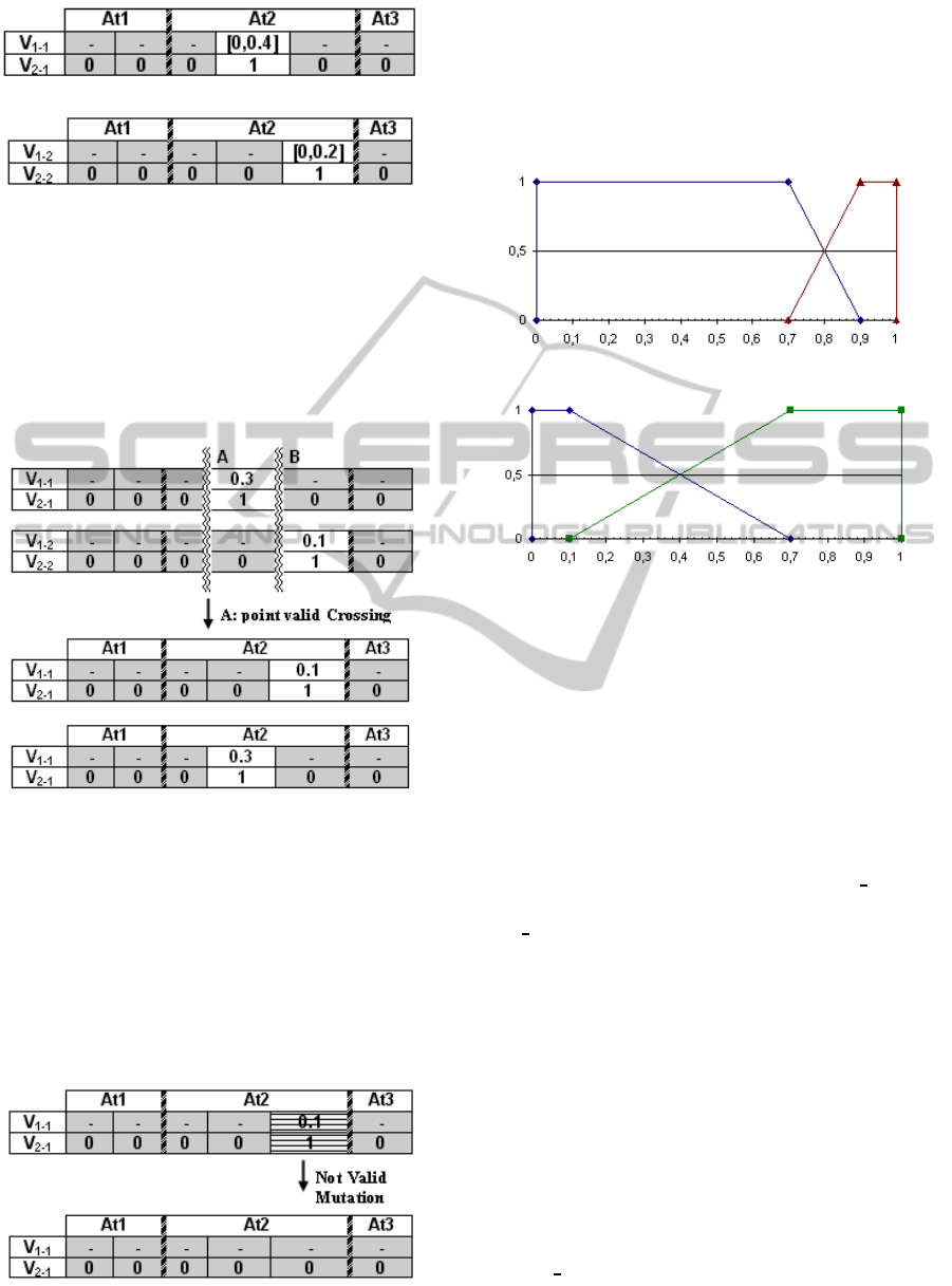
Following with the example given, Figure 2 shows
a possible valid crossing at point A. If the crossing
is realized at point B instead of A, it would not be
valid because the array v
2
would stay with all zero
values and all the split points would be deactivated
and attributes would not be discretized.
Figure 2: Crossing example allowed.
The mutation can generate invalid individuals too.
The Figure 3 shows an example of mutation invalid,
because the individual 2, after the crossing, only has
one active gene and whether this gene is turned off
all genes in array v
2
are zero. If the mutated gene
had been any other, the mutation would be valid. An
important aspect is that if an inactive gene is mutated,
then there are to calculate the domains of the mutated
gene and adjacent.
Figure 3: Mutation example not allowed.
If we assume, in the example, that individuals are
not changed after the crossing shown in Figure 2 and
the algorithm reaches a stopping condition, the algo-
rithm only has discretized the second attribute in the
two individuals. Figure 4 shows the discretization that
each individual makes the second attribute.
a) Discretization of second attribute. Individual 1.
b) Discretization of second attribute. Individual 2.
Figure 4: Fuzzy partition of the example.
This example shows that although in the first stage
many split points are obtained, the algorithm may
only use a subset of these to discretize.
4 EXPERIMENTS
In this section we show several computational re-
sults which measure the accuracy of the OFP CLASS
Algorithm proposed. In order to evaluate the
OFP CLASS Algorithm a comparison with the results
of (Li, 2009) and (Li et al., 2009) is carried out, in
which fuzzy partitions are constructed by means of a
combination of fuzzy clustering algorithms, using the
majority vote rule or the weighted majority vote rule,
respectively. To obtain these results we haveused sev-
eral datasets from the UCI repository (Asuncion and
Newman, 2007), whose characteristics are shown in
Table 2. It shows the number of examples (|E|), the
number of attributes (|A|), the number of continuous
attributes (Cont.) and the number of classes for each
dataset (CL). “Abbr” indicates the abbreviation of the
dataset used in the experiments.
In order to evaluate the partitions generated by
the OFP CLASS Algorithm, we classify the datasets
using the fuzzy decision tree presented in Subsec-
tion 3.2. We compare the results obtained in (Li,
OFP_CLASS: AN ALGORITHM TO GENERATE OPTIMIZED FUZZY PARTITIONS TO CLASSIFICATION
11

Table 2: Datasets description.
Dataset Abbr |E| |A| Cont. CL
Australian Cre. AUS 690 14 6 2
German Cre. GER 1000 24 24 2
Iris Plants IRP 150 4 4 3
Pima Ind. Dia. PIM 768 8 8 2
SPECTF heart SPE 267 44 44 2
Thyroid Dis. THY 215 5 5 3
Zoo ZOO 101 16 1 7
Table 3: Testing accuracies.
Dataset
Best result of
OFP CLASS
(Li, 2009) and (Li et al., 2009)
AUS 60.29% 85.50%±0.00
GER 66.80% 73.13%±0.21
IRP 92.00% 97.33%±0.00
PIM 65.10% 77.07%±0.12
SPE 64.79% 84.09%±0.18
THY 79.07% 95.83%±0.00
ZOO 68.32% 94.06%±0.00
2009) and (Li et al., 2009) with those obtained by
OFP CLASS Algorithm. The comparison is carried
out on the same datasets used in those two references.
For this experiment, a 3×5-fold cross validation was
carried out. In Table 3, the best average success per-
centages obtained in (Li, 2009) and (Li et al., 2009)
and those obtained with OFP CLASS Algorithm are
shown. Also, in the case of OFP CLASS Algorithm
the standard deviation for each dataset is shown.
After the experimental results have been shown,
we perform an analysis of them using statistical tech-
niques. Following the methodology of (Garca et
al., 2009) we use nonparametric tests. We use the
Wilcoxon signed-rank test to compare two methods.
This test is a non-parametric statistical procedure for
performing pairwise comparison between two meth-
ods. Under the null-hypothesis, it states that the meth-
ods are equivalent, so a rejection of this hypothe-
sis implies the existence of differences in the perfor-
mance of all the methods studied. In order to carry
out the statistical analysis we have used R packet.
Results obtained on comparing the OFP CLASS
Algorithm with the best result of (Li, 2009) and (Li
et al., 2009) for each dataset show that, with a 99.9%
confidence level, there are significant differences be-
tween the methods, with the OFP CLASS Algorithm
being the best.
5 CONCLUSIONS
In this study we have presented an algorithm for fuzzy
discretization of continuous attributes, which we have
called OFP CLASS Algorithm. The aim of this algo-
rithm is to find a partition that allows good results to
be obtained when using it afterwards with fuzzy clas-
sification techniques. The algorithm makes use of two
techniques: a Fuzzy Decision Tree and a Genetic Al-
gorithm. Thus the proposed algorithm consists of two
stages, using in the first of them the fuzzy decision
tree to find divisions in the continuous attribute do-
main, and in the second, the genetic algorithm to find,
on the basis of prior divisions, a fuzzy partition.
We have presented experimental results obtained
by applying the OFP CLASS Algorithm to vari-
ous datasets. On comparing the results of the
OFP CLASS Algorithm with those obtained by two
methods in the literature we conclude that the
OFP CLASS Algorithm is an effective algorithm and
it obtains the best results. Moreover, all these conclu-
sions have been validated by applying statistical tech-
niques to analyze the behaviour of the algorithm.
ACKNOWLEDGEMENTS
Supported by the project TIN2008-06872-C04-03 of
the MICINN of Spain and European Fund for Re-
gional Development. Thanks also to the Funding Pro-
gram for Research Groups of Excellence with code
04552/GERM/06 granted by the “Fundaci´on S´eneca”.
REFERENCES
Asuncion, A. and Newman, D. (2007). Uci ma-
chine learning repository. http://www.ics.uci.edu/
mlearn/MLRepository.html.
Au, W.-H., Chan, K. C. C., and Wong, A. K. C. (2006).
A fuzzy approach to partitioning continuous attributes
for classification. IEEE Trans. on Knowl. and Data
Eng., 18(5):715–719.
Bezdek, J. C. (1981). Pattern Recognition with Fuzzy Ob-
jective Function Algorithms. Kluwer Academic Pub-
lishers, Norwell, MA, USA.
Catlett, J. (1991). On changing continuous attributes into
ordered discrete attributes. In EWSL-91: Proceedings
of the European working session on learning on Ma-
chine learning, pages 164–178, New York, NY, USA.
Springer-Verlag New York, Inc.
Cox, E. (2005). Fuzzy Modeling and Genetic Algorithms
for Data Mining and Exploration. Morgan Kaufmann
Publishers.
Cox, E., Taber, R., and OHagan, M. (1998). The Fuzzy
Systems Handbook. AP Professional, 2 edition.
Garca, S., Fernndez, A., Luengo, J., and Herrera, F. (2009).
A study of statistical techniques and performance
ICFC 2010 - International Conference on Fuzzy Computation
12

measures for genetics-based machine learning: accu-
racy and interpretability. Soft Comput., 13(10):959–
977.
Holte, R. C. (1993). Very simple classification rules per-
form well on most commonly used datasets. In Ma-
chine Learning, pages 63–91.
Kbir, M. A., Maalmi, K., Benslimane, R., and Benkirane, H.
(2000). Hierarchical fuzzy partition for pattern classi-
fication with fuzzy if-then rules. Pattern Recogn. Lett.,
21(6-7):503–509.
Li, C. (2009). A combination scheme for fuzzy partitions
based on fuzzy majority voting rule. In NSWCTC
’09: Proceedings of the 2009 International Confer-
ence on Networks Security, Wireless Communications
and Trusted Computing, pages 675–678, Washington,
DC, USA. IEEE Computer Society.
Li, C., Wang, Y., and Dai, H. (2009). A combination scheme
for fuzzy partitions based on fuzzy weighted majority
voting rule. Digital Image Processing, International
Conference on, 0:3–7.
Liu, H., Hussain, F., Tan, C. L., and Dash, M. (2002). Dis-
cretization: An enabling technique. Data Min. Knowl.
Discov., 6(4):393–423.
Piero, P., Arco, L., Garca, M., and Acevedo, L. (2003). Al-
goritmos genticos en la construccion de funciones de
pertenencia borrosas. Revista Iberoamericana de In-
teligencia Artificial, 18:25–35.
Quilan, J. (1993). C4.5: Programs for Machine Learning.
Morgan Kaufmann Publishers.
OFP_CLASS: AN ALGORITHM TO GENERATE OPTIMIZED FUZZY PARTITIONS TO CLASSIFICATION
13
