PROLONGATION RECOGNITION IN DISORDERED SPEECH

USING CWT AND KOHONEN NETWORK

Ireneusz Codello, Wiesława Kuniszyk-Jóźkowiak, Elżbieta Smołka and Adam Kobus

Institute of Computer Science, Maria Curie-Skłodowska University, pl. Marii Curie-Skłodowskiej 1, Lublin, Poland

Keywords: Kohonen network, Automatic prolongation recognition, Waveblaster, Neuron reduction, CWT, Continuous

wavelet transform, Bark scale.

Abstract: Automatic disorder recognition in speech can be very helpful for the therapist while monitoring therapy

progress of the patients with disordered speech. In this article we focus on prolongations. We analyze the

signal using Continuous Wavelet Transform with 22 bark scales, we divide the result into vectors (using

windowing) and then we pass such vectors into Kohonen network. We have increased the recognition ratio

from 54% to 81% by adding a modification into the network learning process as well as into CWT

computation algorithm. All the analysis was performed and the results were obtained using the authors’

program – “WaveBlaster”. It is very important that the recognition ratio above 80% was obtained by a fully

automatic algorithm (without a teacher). The presented problem is part of our research aimed at creating an

automatic prolongation recognition system.

1 INTRODUCTION

Speech recognition is a very important branch of

informatics nowadays – oral communication with a

computer can be helpful in real-time document

writing, language translating or simply in using a

computer. Therefore the issue has been analyzed for

many years by researches, which caused many

algorithms to be created such as Fourier transform,

Linear Prediction, spectral analysis. Disorder

recognition in speech is quite a similar issue – we try

to find where speech is not fluent instead of trying to

understand the speech, therefore the same algorithms

can be used. Automatically generated statistics of

disorders can be used as a support for therapists in

their attempts at an estimation of the therapy

progress.

We have decided to use a relatively new

algorithm – Continuous Wavelet Transform (CWT)

(Akansu and Haddar 2001, Coddello and Kuniszyk-

Jóźkowiak 2007, Nayak 2005), because by using it

we can choose scales (frequencies) which are most

suitable for us (Fourier transform and Linear

Prediction are not so flexible). We have choosen the

bark scales set, which is, besides the Mel scales and

the ERB scales, considered as a perceptually based

approach (Smith and Abel 1999). The CWT result

is divided into fixed-length windows, each one is

converted into a vector and such a vector is passed

into the Kohonen network. Then we use a simple

algorithm on the Kohonen output to determine if this

window contains prolongation or not. This way we

obtain the list of the windows in which

prolongations occurred.

After creating recognition statistics we decided

to add a few algorithm improvements which

signifficantly increased the recognition ratio.

2 CWT

2.1 Mother Wavelet

Mother wavelet is the heart of the Continuous

Wavelet Transform.





baba

ttxCWT )()(



(1)



















)(

(2)

where x(t) – input signal, ψ

a,b

(t) – wavelet family,

ψ(t) – mother wavelet, a – scale (multiplicity of

mother wavelet), b – offset in time.

392

Codello I., Kuniszyk-JóÅžkowiak W., Smołka E. and Kobus A..

PROLONGATION RECOGNITION IN DISORDERED SPEECH USING CWT AND KOHONEN NETWORK.

DOI: 10.5220/0003057903920398

In Proceedings of the International Conference on Fuzzy Computation and 2nd International Conference on Neural Computation (ICNC-2010), pages

392-398

ISBN: 978-989-8425-32-4

 2010 SCITEPRESS (Science and Technology Publications, Lda.)

We used Morlet wavelet of the form

(Goupillaud, Grossmann, Morlet, 1984-1985):

)202cos()(

tet









(3)

which has center frequency F

=20Hz. Mother

wavelets have one significant feature: length of the

wavelet is connected with F

which is a restraint for

us. Morlet wavelet is different because we can

choose its length and then set its F

by changing the

cosines argument.

2.2 Scales

For frequencies of scales we decided to assume a

perceptually based approach – because it is

considered to be the closest to the human way of

hearing. We choose Hartmut scales (Traunmüller

1990):

53.0

/19601

81.26







, f – freq. in Hz

(4)

The frequency of each wavelet scale a was

computed from the equation

aFFF

SCa

/ , F

– sampling frequency

(5)

Due to the discrete nature of the algorithm, it was

not always possible to match scale a with scale B

perfectly (Table 1).

Table 1: 22 scales a (and scale’s shift b) with

corresponding frequencies f and bark scales B.

a [scale] f [Hz] B [bark] b [samples]

46 9586 21,7 23

57 7736 20,9 29

68 6485 20,1 34

83 5313 19,1 42

100 4410 18 50

119 3705 17 60

140 3150 16 70

163 2705 15 82

190 2321 14 95

220 2004 13 110

256 1722 12 128

297 1484 11 149

347 1270 10 174

408 1080 9 204

479 920 8 240

572 770 7 286

700 630 6 350

864 510 5 432

1102 400 4 551

1470 300 3 735

2205 200 2 1103

4410 100 0,8 2205

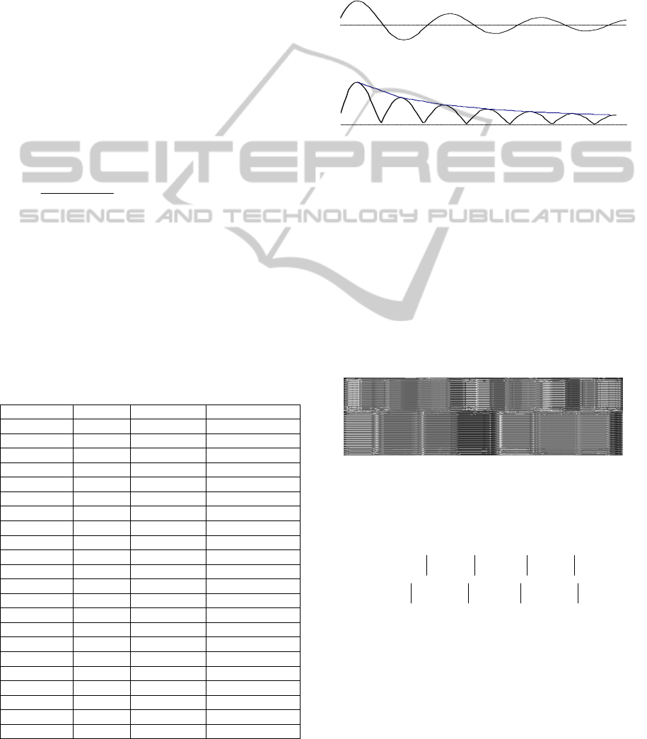
2.3 Smoothing Scales

Because CWT values are similarity coefficients

between signal and wavelet, we assumed that the

sign of its value is irrelevant, therefore in all

computations modules are taken – |CWT

a,b

|. We

went one step further and we smoothed the |CWT

a,b

by creating a contour (see Figure 2)

Figure 1: Cross-section of one CWT

a,b

scale.

Figure 2: Cross-section of one |CWT

a,b

| scale and its

contour (smoothed version).

2.4 Windowing

Thus now we have spectrogram consisting of 22

smoothed bark scales vectors. Then we cut the

spectrogram into 23.2ms frames (512 samples when

=22050Hz), with a 50% frame offset. Because

every scale has its own offset – one window of fixed

width (e.g. 512 samples) will contain different

number of amplitudes (CWT similarity coefficients)

in each scale (see Figure 3), therefore we take the

arithmetic mean of each scale's amplitudes.

Figure 3: One CWT window (512 samples when

=22050Hz).

From one window we obtain the vector V of the

form:



 





44102205

5746

,...,

CWTmeanCWTmean

CWTmeanCWTmeanV 



(6)

Such consecutive vectors are then passed into the

Kohonen network.

3 KOHONEN NETWORK

The Kohonen network (Kohonen T, 2001, Garfield

PROLONGATION RECOGNITION IN DISORDERED SPEECH USING CWT AND KOHONEN NETWORK

393

S. 2001) (or "self-organizing map", or SOM, for

short) was developed by Teuvo Kohonen. The basic

idea behind the Kohonen network is to establish a

structure of interconnected processing units

("neurons") which compete for the signal. While the

structure of the map may be quite arbitrary, we use

rectangular maps.

Let assume that:

 Kohonen network has K neurons

 n is dimension of each input vector X

 each element

 is connected to all K

neurons, so we have

nK  connections. Every

connection is represented by it’s weight w

i=1..n, j=1..K which are adjusted during the

training.

We use the Kohonen network to convert 3-

dimention CWT spectrogram into 2-dimention

winning neuron contour (Szczurowska and

Kuniszyk-Jóźkowiak, 2006, 2007)

3.1 Learning Algorithm

The basic training algorithm is quite simple:

 select the input vector from the training set – we

could take consecutive vectors, or take them

randomly

 find the neuron which is closest to the given

input vector (i.e. the distance between





niwW

ijj

..1:  and X is a minimum). The

metric can be arbitrary, usually Euclidean, where

the distance between the input vector and i-th

neuron is defined:









ijji

wxd

(7)

 adjust the weight vectors of the closest node and

the nodes around it in a way that they move

towards the training data:





jjj

WXWW









(8)

, α is a coefficient factor, usually connected with the

distance from the winning neuron

 repeat all steps for a fixed number of repetitions

As a result of such learning, we can say that, in a

Kohonen map, neurons located physically next to

each other will correspond to classes of input vectors

that are likewise next to each other (Figure 4).

Therefore such regions are called maps.

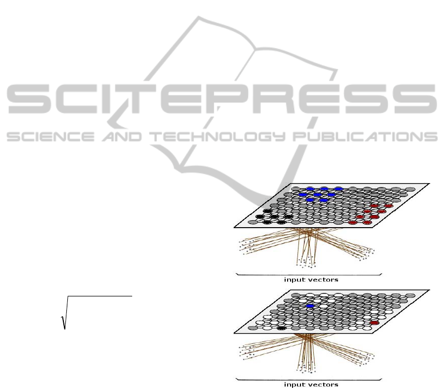
3.2 Learning Algorithm Modification

We added one additional step into the learning

process (Codello and Kuniszyk-Jóźkowiak 2010).

This step is applied after the network has been

trained using the standard algorithm described

previously. The purpose is to reduce each map

(which contains similar neurons) to only one neuron

within one map.

We do the following:

 Find two closest neurons k

, k

(the distance

between neurons weights are measured using

Euclidean metric – equation 7.)

 If the distance is less then some threshold

(algorithm’s parameter), fill weights of one of

the neurons with zeros. This way input vectors

that were assigned to k

neuron, now will be

assigned to k

 Repeat steps 1. and 2. until there exists a pair of

neurons closer then the threshold.

The result of the reducing procedure is shown in

Figures 5 and 6. As we can see, such a result is

much clearer and therefore more useful than an

unmodified result.

Figure 4: Input vectors with corresponding maps on

Kohonen network before (top) and after (bottom) "neuron

reduction". Similar vectors are assigned to group of

neurons (top) and to only one neuron (bottom). Other

neurons (white ones) within the maps are cleared.

ICFC 2010 - International Conference on Fuzzy Computation

394

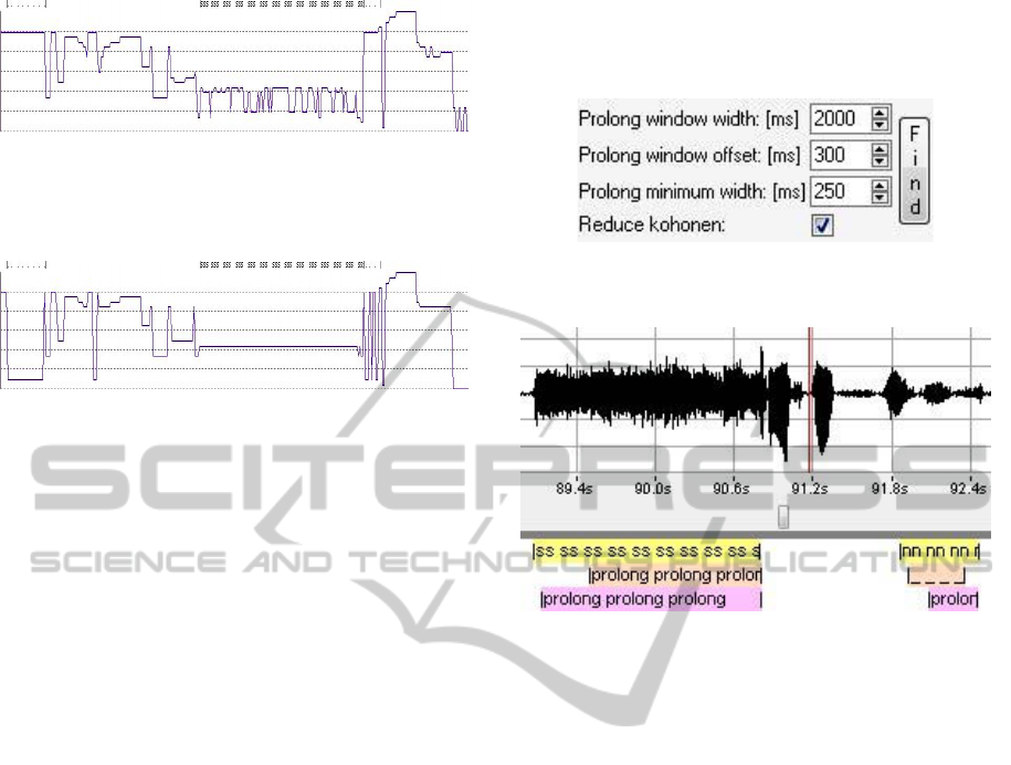
Figure 5: Winning neuron contour of the 2 seconds long

utterance with prolongation “sss”. Kohonen network size:

5x5. Vertical axis: winning neuron number, horizontal

axis: time. Screenshot from program “WaveBlaster”.

Figure 6: Winning neuron contour from Figure 5 after

"neuron reduction". Screenshot from program

“WaveBlaster”.

4 AUTOMATIC PROLONGATION

RECOGNITION

The procedure of finding prolongations in the file is

the following:

 Compute CWT spectrogram for the entire file

 Divide the spectrogram into ‘small’ windows

(e.g. 23.2 ms) with a certain offset (e.g. 11.6 ms).

By using windowing (see section 2.4 for details)

each ‘small’ window is converted into a set of 22

element vectors (each vector’s element

corresponds to one bark scale)

 Divide the result into ‘big’ windows (e.g.

2000ms – first parameter on Figure 7) with a

certain shift (e.g. 300ms – second parameter on

Figure 7)

 Each window, which consists of 22-element

vectors, is passed into the Kohonen network.

After the learning process we obtain a winning

neuron graph (Figure 5)

 Then we can perform the Kohonen neuron

reduction (fourth option in Figure 7)

 If a winning neuron contour (Figure 6) contains a

section longer then a certain parameter (e.g.

250ms – the third parameter in Figure 7) in

which only one neuron wins – then this section is

considered as prolongation

 If the section overlaps some other automatically

found prolongation, then the sections are

combined

 At the end we manually compare the pattern with

the algorithm output and count the number of

correctly and incorrectly recognized prolongation

(Figure 8)

Figure 7: Automatic prolongation options panel.

Screenshot from program “WaveBlaster”.

Figure 8: Input signal with three sets of patterns (first one

manually created, other two automatically generated by

algorithm with different configuration) – screenshot from

program WaveBlaster.

5 WAVEBLASTER

The presented way of Kohonen post-learning and

CWT smoothing is quite unique, therefore we had to

create our own tool for this purpose. The presented

problem is only part of our research (an automatic

prolongation recognition system) – therefore our

program ’WaveBlaster’ has quite a developed

functionality and set of parameters.

The following algorithms are implemented:

 DTF, iDFT, FFT, iFFT

 FFT reduced by 1/3 octave filters

 Linear Prediction (LP)

 Formant tracking (based on LP)

 Vocal tract visualization (based on LP)

 Signal envelope calculation

 DWT, CWT

 Kohonen neural network

 Automatic

The following graphs are displayed:

 DFT, FFT, 1/3 octave FFT, LP, DWT and CWT

PROLONGATION RECOGNITION IN DISORDERED SPEECH USING CWT AND KOHONEN NETWORK

395

 2D spectrums and 3D spectrograms

 LP parameters and formant paths

 3D vocal tract visualization

 Kohonen neural network

 Wavelets and wavelet scales

All the modules, despite of the numerous

elements, are consistent. The components are

flexibly programmed, enabling the user to easily

change and visualize the data – which is very useful

in research processes during which, when we look

for the answers and some regularity, we need to look

at the same set of data from different perspectives

(enlarging, reducing, shifting, selecting, changing

colors, scales, different analysis). The precise system

of axis scales and variety of quantity measurement is

very helpful in the observation process and finding

even small irregularities in data behavior. All graphs

are connected to each other (enlarging, reducing,

shifting and selecting affects all panels) and

therefore for a particular fragment we can observe

many coefficients simultaneously (oscillogram,

spectrograms, spectrums) – which is also quite

helpful while doing research.

Summarizing – all these features make our

application a very useful research tool. It is focused

only on a particular sort of computation – which is

both an advantage and a disadvantage. All this can

be done by other tools, like MATLAB, but we

would not have been able to do it so quickly and

comprehensively (in the context of our needs).

Therefore we think that despite the effort made to

implement this tool, it was worth it – it will be used

in many situations, facilitating and speeding up the

research.

6 RECOGNITION EFFICIENCY

ANALISYS

6.1 Input Data

We took Polish disordered speech recordings of 6

persons and Polish fluent speech recordings of 4

persons. In the disordered speech recordings we

chose all prolongations with 4 seconds surroundings

and from fluent speech we randomly chose several 4

seconds long sections. We merged all the pieces

together obtaining 15 min 24 s long recording

containing 286 prolongations. The statistics are the

following:

Table 2: Prolongations count.

all

286

6.2 Algorithm Parameters

In CWT we used Morlet wavelet (equation 3) with

22 Hartmut bark scales (Table 1).

Vectors for the Kohonen network were created

from CWT spectrogram frames divided into 23.2ms

windows shifted by 50% of frame length (11.6 ms) –

for details see paragraph 2.4.

We used a 5x5 Kohonen network with the

following learning parameters: 100 epochs, learning

coefficient 0.10-0.10, neighbor distance 1.5-0.5,

reducing distance 0.30.

An automatic prolongation recognition algorithm

was run with the following settings: prolongation

window equal 2s, offset equal 300ms and minimum

prolongation equal 250ms.

The recognition ratio was calculated using the

formulas (Barro and Marin 2002):

litypredictabi

ysensitivit





(9)

where P is the number of correctly recognized

prolongations, A is the number of all prolongations

and B is the number of fluent sections mistakenly

recognized as prolongation.

6.3 Results

We wanted to test the following two issues:

 how the neuron reducing algorithm (see section

3.2 for details) influences the recognition ratio

 how the CWT smoothing algorithm (see section

2.3 for details) influences the recognition ratio

Therefore we performed the following four tests:

 CWT smoothing: NO, Kohonen network neuron

reduction: NO

 CWT smoothing: NO, Kohonen network neuron

ICFC 2010 - International Conference on Fuzzy Computation

396

reduction: YES

 CWT smoothing: YES, Kohonen network neuron

reduction: NO

 CWT smoothing: YES, Kohonen network neuron

reduction: YES

The results are presented in Table 3.

Table 3: Automatic prolongation recognition results.

1. CWT smoothing – NO, Kohonen reduction – NO

A P B

sensitivity predictability

286 154 8

54% 95%

2. CWT smoothing – NO, Kohonen reduction – YES

A P B

sensitivity predictability

286 179 12

63% 94%

3. CWT smoothing – YES, Kohonen reduction – NO

A P B

sensitivity predictability

286 213 44

74% 83%

4. CWT smoothing – YES, Kohonen reduction – YES

A P B

sensitivity predictability

286 231 48

81% 83%

7 CONCLUSIONS

As we can see, the CWT smoothing algorithm

increased the recognition ratio from 54% (set 1.) to

74% (set 3.) and from 63% (set 2.) to 81% (set 4.). It

gives us 20% and 18% – that is very good. The

CWT algorithm is too precise – especially in the hi-

frequency scales. For the prolongation finding

purpose such precision it is too high – that is why

smoothing gives such a good ratio improvement.

The disadvantage of this method is that it decreases

predictability by 12% (set 1 and 3) and 11% (set 2

and 4), therefore it needs to be improved.

The Kohonen neuron reduction algorithm is a

little more difficult to interpret. We used such an

algorithm because if a prolongation is long (e.g.

1000ms), then consecutive vectors within that period

are similar to each other – they represent one

phoneme. We observed that when we want to have

only one winning neuron for that phoneme, then

other neurons have to compete for other phonemes,

therefore

 A) all input vectors representing the prolongation

have to be almost identical, then no matter how

big the network, only one neuron will win the

competition for the prolongation phoneme or

 B) an input signal needs to have a few other pho-

nemes in the window (proportional to the size of

the network) – then every neuron in the network

will compete for a different phoneme

When a given prolongation is short, then usually

there are a few phonemes within the window,

therefore condition B is met, which is good. But if

the prolongation is long, or there is a lot of silence,

then there are not many phonemes in the window.

The Kohonen neurons start to compete for the same

phoneme and they specialize in different variations

of one phoneme, which is bad because we want only

one neuron to win. That is why the CWT smoothing

algorithm works so well – it makes similar vectors

even more similar to each other and then condition A

is met. And that is why the ‘neuron reduction’

algorithm is working – it reduces excessive neurons

(condition B is met).

As we can see, ‘neuron reduction’ increases the

recognition ratio by 9% (set 1 and 2) and by 7% (set

3 and 4), which is significant. What is important is

that it does not reduce predictability – it means that

the algorithm improves recognition without

increasing the number of algorithm mistakes.

The results are promising. Now the main issues

are:

 to improve the CWT smoothing algorithm – it

decreases predictability ratio too much

 to investigate the Kohonen learning parameters

for better prolongation recognition such as: the

Kohonen network size, Kohonen network

learning and neighbour coefficients, Kohonen

network neuron initialization method, wavelet

scales and scale shifts, decibel threshold. The

research into the parameters is in progress.

REFERENCES

Akansu A.N, Haddad R. A., 2001, Multiresolution signal

decomposition, Academic Press.

Barro S., Marin R., 2002, Fuzzy Logic in Medicine,

Physica-Verlag Heidenberg, New York

Codello I., Kuniszyk-Jóźkowiak W., 2007, Wavelet

analysis of speech signal, Annales UMCS Informatica,

2007, AI 6, Pages 103-115.

Codello I., Kuniszyk-Jóźkowiak W., Kobus A., 2010,

Kohonen network application in speech analysis

algorithm, Annales UMCS Informatica, (Accepted

paper).

Garfield, S., M. Elshaw, and S. Wermter. 2001, Self-

orgazizing networks for classification learning from

normal and aphasic speech. In The 23rd Conference of

the Cognitive Science Society. Edinburgh, Scotland

Gold, B., Morgan, N., 2000. Speech and audio signal

PROLONGATION RECOGNITION IN DISORDERED SPEECH USING CWT AND KOHONEN NETWORK

397

processing, JOHN WILEY & SONS, INC.

Goupillaud P., Grossmann A., Morlet J., 1984-

1985.`Cycle-octave and related transforms in seismic

signal analysis'', Geoexploration, 23, 85-102

Huang, X., Acero, A., 2001. Spoken Language Processing:

A Guide to Theory, Algorithm and System

Development, Prentice-Hall Inc.

Kohonen, T., 2001, Self-Organizing Maps, 34:p.2173-

2179

Nayak J., Bhat P. S., Acharya R., Aithal U. V., 2005,

Classification and analysis of speech abnormalities,

Volume 26, Issues 5-6, Pages 319-327, Elsevier SAS

Smith J., Abel J, 1999, Bark and ERB Bilinear

Transforms, IEEE Transactions on Speech and Audio

Processing, November, 1999.

Szczurowska, I, W. Kuniszyk-Jóźkowiak, and E. Smołka,

2006,The application of Kohonen and Multilayer

Perceptron network in the speech nonfluency analysis.

Archives of Acoustics. 31 (4 (Supplement)): p. 205-

210

Szczurowska, I, W. Kuniszyk-Jóźkowiak, and E. Smołka,

2007, Application of Artificial Neural Networks In

Speech Nonfluency Recognition. Polish Jurnal of

Environmental Studies, 2007 16(4A): p. 335-338.

Traunmüller H., 1990 "Analytical expressions for the

tonotopic sensory scale" J. Acoust. Soc. Am. 88: 97-

100.

ICFC 2010 - International Conference on Fuzzy Computation

398