
A NOVEL ADAPTIVE CONTROL VIA SIMPLE RULE(S) USING
CHAOTIC DYNAMICS IN A RECURRENT NEURAL NETWORK
MODEL AND ITS HARDWARE IMPLEMENTATION
Ryosuke Yoshinaka
1
, Masato Kawashima
1
, Yuta Takamura
1
, Hitoshi Yamaguchi
1
Naoya Miyahara
1
, Kei-ichiro Nabeta
1
, Yongtao Li
2
and Shigetoshi Nara
1
1
Graduate School of Natural Science and Technology, Okayama University
3-1-1 Tsushima-naka, Kita-ku, Okayama 700-8530, Japan
2
Research Institute for Electronic Science, Hokkaido University, Kita 12-jyo Nishi 7-chome, Kita-ku, Sapporo, Japan
Keywords:
Dynamics, Adaptive control, Recurrent neural network, Hardware implementation, Autonoumous robot, Neu-
romorphic device, Brainmorphic device.
Abstract:
A novel idea of adaptive control via simple rule(s) using chaotic dynamics in a recurrent neural network model
is proposed. Since chaos in brain was discovered, an important question, what is the functional role of chaos
in brain, has been arising. Standing on a functional viewpoint of chaos, the authors have been proposing that
chaos has complex functional potentialities and have been showing computer experiments to solve many kinds
of ”ill-posed problems”, such as memory search and so on. The key idea is to harness the onset of complex
nonlinear dynamics in dynamical systems. More specifically, attractor dynamics and chaotic dynamics in a
recurrent neural network model are introduced via changing a system parameter, ”connectivity”, and adaptive
switching between attractor regime and chaotic regime depending surrounding situations is applied to realiz-
ing complex functions via simple rule(s). In this report, we will show (1)Global outline of our idea, (2)Several
computer experiments to solve 2-dimensional maze by an autonomous robot having a neural network, where
the robot can recognize only rough directions of target with uncertainty and the robot has no pre-knowledge
about the configuration of obstacles (ill-posed setting), (3)Hardware implementations of the computer experi-
ments using two-wheel or two-legs robots driven by our neuro chaos simulator. Successful results are shown
not only in computer experiments but also in practical experiments, (4)Making pseudo-neuron device using
semiconductor and opto-electronic technologies, where the device is called ”dynamic self-electro optical effect
devices (DSEED)”. They could be ”neuromorphic devices” or even ”brainmorphic devices”.
1 INTRODUCTION
Since chaos is discovered in many natural phenom-
ena, particularly, chaotic dynamics observed in bi-
ological systems including brain suggest us to con-
sider whether there are certain important relations be-
tween chaotic dynamics and their excellent functions
in both information processing and well-regulated
functioning or controlling. (Skarda and Freeman,
1987)(Tsuda, 2001)(Fujii et al., 1996)(Tokuda et al.,
1997).
On the other hand, the rapid progress of robotics
have brought various robots into our life and indus-
try, however, it is still quite difficult for the robots
to perform tasks adaptively in various environments,
whereas biological systems have excellent functions
in both information processing and well-regulated
functioning in various environments. Conventional
methodologies (decomposing a system into parts and
elements) often fall into difficulties to face enor-
mous complexity originating from dynamics in sys-
tems with large but finite degrees of freedom.
Under these situations, biological information and
control processing has suggested that they could work
under novel dynamical mechanism that cause excel-
lent functions in information processing and/or con-
trolling. Therefore, many dynamical models have
been proposed for approaching the mechanisms by
means of large-scale simulation or heuristic meth-
ods. Our work originates from a novel idea to har-
ness the onset of complex nonlinear dynamics in in-
formation processing or control systems, and mainly
study chaotic dynamics in neural networks from the
functional viewpoint. First, Nara & Davis intro-
145
Yoshinaka R., Kawashima M., Takamura Y., Yamaguchi H., Miyahara N., Nabeta K., Li Y. and Nara S..
A NOVEL ADAPTIVE CONTROL VIA SIMPLE RULE(S) USING CHAOTIC DYNAMICS IN A RECURRENT NEURAL NETWORK MODEL AND ITS
HARDWARE IMPLEMENTATION .
DOI: 10.5220/0003058301450155
In Proceedings of the International Conference on Fuzzy Computation and 2nd International Conference on Neural Computation (ICNC-2010), pages
145-155
ISBN: 978-989-8425-32-4
Copyright
c
2010 SCITEPRESS (Science and Technology Publications, Lda.)

duced chaotic dynamics into a recurrent neural net-
work model (RNNM) by adjusting only one system
parameter (connectivity among neurons), and they
proposed that constrained chaos could be potentially
useful dynamics to solve complex problem, such as
ill-posed problems (Nara and Davis, 1992). As one
of functional experiments, chaotic dynamics was ap-
plied to solving a memory search task or image syn-
thesis which is set in an ill-posed context (Nara et al.,
1993)(Nara et al., 1995)(Nara, 2003). Furthermore,
the idea is extended to challenging application of
chaotic dynamics to control. Chaotic dynamics in-
troduced in a recurrent neural network model was
applied to control tasks that an object is requested
to solve a two-dimensional maze for catching a tar-
get (Suemitsu and Nara, 2004), or to capture a tar-
get moving along different trajectories (Li and Nara,
2008). From the results of computer experiments,
we consider that complex dynamics/chaotic dynamics
could be useful not only in solving ill-posed problems
but also in controlling of systems with large but finite
degrees of freedom.
Therefore, in the present paper, we develope our
idea and propose a quasi-layered RNNM consist-
ing of sensing neurons(upper layer) and driving neu-
rons(lower layer). In both layers, chaotic dynamics
are used. This idea is based on the work of Mikami
and Nara who found that chaos has a sensitive re-
sponse property to external input (Mikami and Nara,
2003). Their idea is applied to practical functional ex-
periments to solve 2-dimensional mazes, as shown in
the later sections. We can find a corresponding exam-
ple in biological behaviors. For instance, auditory be-
havior of cricket gives a typical ill-posed problem in
biological systems (Huber and Thorson, 1985). Fur-
ther developments are shown about the following top-
ics. They are:
(a) to apply our idea to a roving robot with two legs;
(b) to apply our idea to an arm robot;
(c) to propose a hardware device of pseudo-neuron
and a network of them, and to evaluate them by
computer experiments;
(c) to make an actual hardware device using semicon-
ductor and opto-electronic technologies.
2 CONTROL SYSTEM
2.1 Construction of Control System
The control system mainly consists of a roving robot
with a micro processor unit (MPU), sensing systems
of sound signal from target and of detecting obsta-
cles, a neural chaos simulator, Bluetooth interface be-
tween the robot and the neural chaos simulator, and
a target emitting a specified sound signal, which is
like a singing male cricket, shown as Fig.1. The
Figure 1: Block diagram of control system.
robot with sensors is shown as Fig.2. It has two driv-
ing wheels and one castor (2DW1C). The robot has
six sensors which can be divided into two parts. One
is the sensing system of detecting obstacles that con-
sists of two ultrasonic sensors which givethe robot the
ability to detect whether an obstacle does exist in front
of the robot without actually touching it. The other is
the sensing system of sound signal from target that
consists of four sets of directional microphone cir-
cuits, which functions as ears of the robot. Four mi-
crophones are set with directing to the front, the back,
the left and the right of the robot, which is shown as
Fig.2(right). In our study, a loud speaker is employed
as the target, and is emitting 3.6KHz sound signal
like a singing cricket. This sound signal is picked
up by these four ears(microphone) with π/2 detect-
ing angle oriented to four directions. Among them,
a sound signal coming from one side might have a
strongest intensity, or be loudest. These four sound
signals are amplified, rectified , digitalized, and trans-
ferred to MPU, respectively. At the preliminary stage,
these signals are used to compare which direction is
the strongest one. In near future, we will try to in-
put them into sensing neurons (upper layer) in quasi-
layered RNNM, but in the present study, we must em-
phasize the two points. One is that, the sensing sys-
tem of sound signal from target does not give accu-
rate directional information of target, but rough di-
rectional information of target with uncertainty. The
other is that, these signals inputted from four micro-
phones are not processed with complex techniques
or methods. These are quite important differences
between our work and other conventional robotics.
Now, the problem is how these sensing signals
are sent to the neural chaos simulator, which works
as the neural network system to make adaptive be-
haviors of the robot. In our study, a computer with
good performance is chosen as the neural chaos simu-
lator, which is programmed in C language and works
in Vine Linux. A wireless communication interface
ICFC 2010 - International Conference on Fuzzy Computation
146

Figure 2: The roving robot with sensors including two ultra-
sonic sensors and four microphones: A photo picture (left)
and a sketch map (right).
between the MPU of the robot and the neural chaos
simulator has been built using a pair of Bluetooth
serial adapter and a group of communication proto-
col. After the sensing signals was sent to the neural
chaos simulator, the simulator performs neural infor-
mation processing, produces adaptive motion signals,
and sends them back to the robot again. And then, the
robot moves one step. At a new position, sensing in-
formation from sensors are checked again. The above
process is repeated. Therefore, this is a close-loop
control system. After the sensing systems and com-
munication interface have worked well, it is the key
point whether the neural simulator enables the robot
to produce adaptive motions in various environment,
such as mazes or moving targets. In next section, we
will introduce it in detail.
2.2 Context Setting of Solving Mazes
In the present study, the context setting of solving
mazes is shown as follows.
1) Set a typical ill-posed problem of solving two-
dimensional mazes.
2) Set obstacles unknown by the robot.
3) Set a target emitting a sound signal.
4) Acquire information for reaching the target.
•Check whether obstacles to preventthe robot from
forward moving exist or not, by ultrasonic sensors for
detection.
• Obtain rough direction of the target by four mi-
crophones.
5) Calculate the motion increments at every time
step of updating neural network activity.
3 NEURAL CHAOS SIMULATOR
The neural chaos simulator is utilized to simulate dy-
namical activities of neural network, and works like
the ”brain” of the robot. In various unknown en-
vironment or mazes, chaotic dynamics generated in
the neural network makes the robot generate complex
motions to adapt environment or avoid obstacles. In
our study, we start from a simple RNNM, and de-
velop it to a quasi-layered RNNM so as to approach
the mechanism of brain nearer.
3.1 Recurrent Neural Network Model
Our study works with a fully interconnected RNNM
consisting of N binary neurons, and the updating rule
is defined by
S
i
(t + 1) = sgn
∑
j∈G
i
(r)
W
ij
S
j
(t)
(1)
sgn(u) =
+1 u ≥0;
−1 u < 0.
• S
i
(t) = ±1(i = 1 ∼N) : the firing state of a neuron
specified by index i at time t.
• W
ij
: connection weight from the neuron S
j
to the
neuron S
i
, W
ii
is taken to be 0.
• r(0 < r < N): fan-in number for neuron S
i
, named
connectivity
• G
i
(r): spatial configuration set of connectivity r
for neuron S
i
At a certain time t, the state of neurons in the network
can be represented as a N-dimensional state vector
S(t), called as state pattern. The updating rule shows
that time developmentof state pattern S(t) depends on
the connection weight matrix W
ij
and connectivity r.
Therefore, when full connectivityr = N−1, by means
of a kind of orthogonalized learning method (Nara
et al., 1995) , appropriately determiningW
ij
could em-
bed a group of N dimensional state pattern as cyclic
memory attractors in N dimensional state space. At-
tractor patterns consists of (K patterns per cycle)× L
cycles, and each patterns has N neurons. For exam-
ple, in Fig.3, we take K = 6, L = 4,and N = 400. In
this case, the firing states of N = 20×20 = 400 neu-
rons are represented by black pixel or white pixel. As
the network evolves with the updating rule for enough
time steps, randomly initial state pattern will converge
into one of embedded cyclic attractors. Now we
Figure 3: One example of embedded attractor patterns:
when connectivity r = N −1, if S(t) is ξ
1
1
, then the output
sequence is ξ
2
1
, ξ
3
1
,..., ξ
6
1
, ξ
1
1
,....
A NOVEL ADAPTIVE CONTROL VIA SIMPLE RULE(S) USING CHAOTIC DYNAMICS IN A RECURRENT
NEURAL NETWORK MODEL AND ITS HARDWARE IMPLEMENTATION
147
reduce connectivity r by blocking signal transfer from
other neurons, attractors gradually becomes unstable,
and the network state changes from attractor dynam-
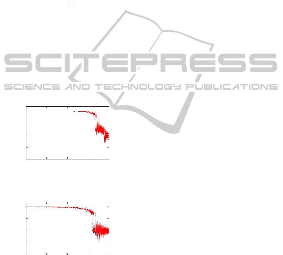
ics to chaotic dynamics. In order to analyze the desta-
bilizing process, we have calculated a bifurcation di-
agram of overlap (Fig.4) where overlap means one-
dimensional projection of state pattern S(t) to a cer-
tain reference pattern. Therefore, an overlap m(t) is
defined by
m(t) =
1
N
S(0) ·S(t) (2)
t = Kp+ t
0
(p = 1,2,. . .) (3)
where S(0) is an initial pattern(reference pattern) and
S(t) is the state pattern at time step t. Because m(t) is
a normalized inner product, −1 ≤m(t) ≤ 1. m(t) = 1
means that the present state pattern and the reference
pattern is same. In other words, the reference pattern
repeatedly appears every K=6 steps. In our study, for
the upper layer and the lower layer, we have calcu-
lated the overlap m(t) with respect state pattern S(t)
when it evolves for long time.
-1
-0.5
0
0.5
1
0 100 200 300 400
m(t)
Overlap
r(r
u,u
)Connectivity
Figure 4: The long-time behaviours of overlap m(t) at K-
step mappings. The horizontal axis is r(r
u,u
) (0-399).
-1
-0.5
0
0.5
1
0 100 200 300 400
r
l,l
Connectivity
m
l
(t)Overlap
Figure 5: The long-time behaviors of overlap m
l
(t) at K-
step mappings (r
u,l
= 0). The horizontal axis is r
l,l
(0-399).
3.2 Quasi-layered Recurrent Neural
Network Model
A quasi-layered RNNM consists of a upper layer with
N neurons and a lower layer with N neurons. The
upper layer is updated by only self-recurrence. On
the other hand, the lower layer are updated not only
by self-recurrence but also by recurrent outputs of the
upper layer. State pattern S(t) = [x(t),y(t)], where
x(t) = {x
i
(t) = ±1 | i = 1,2,··· , N} and y(t) =
{y
i
(t) = ±1 | i = 1, 2,··· ,N}. The updating rules
of two layers are defined by
x
i
(t + 1) = sgn
∑
j∈G
u
(r
u
)
W
u−u
ij
x
j
(t)
(4)
y
i
(t + 1) = sgn
∑
j∈G
l
(r
l
)
[W
l−l
ij
y
j
(t) +W
u−l
ij
x
j
(t)]
,(5)
where u means upper layer, l, lower layer, respec-
tively. W
u−u
ij
is connection weight from neuron x
j
of upper layer to neuron x
i
of upper layer, W
u−l
ij
and
W
l−l
ij
are defined similarly.
In quasi-layered RNNM, if we take sufficiently
large connectivity r (r
u,u
≃ N,r
u,l
≃ N,r
l,l
≃ N), by
appropriately determining connection weight W
ij
, a
group of arbitrarily designed state patterns can be em-
bedded as cyclic memory attractors. Certain cyclic
memory attractors are embedded in each layer. Since
three connectivities r
uu
, r
ul
, r
ll
affect the development
of state pattern, for the upper layer and the lower
layer, we have calculated the overlap m(t) with re-
spect state pattern S(t) when it evolves for long time.
The overlap m
u
(t) of the upper layer as a function of
connectivity r
u,u
is same to Fig.4.
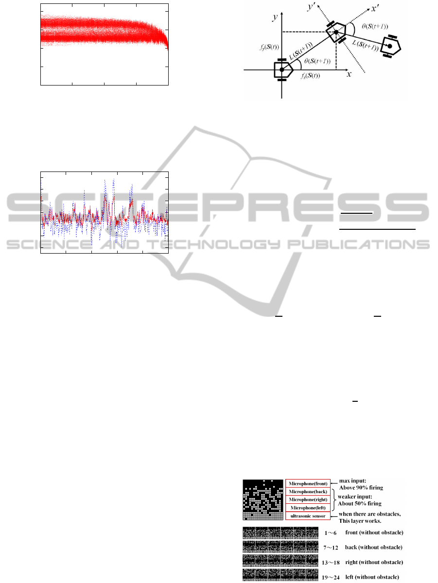
Next, let us show examples about long time be-
haviors of m
l
(t) for a few cases of connectivities, r
uu
,
r
ul
, r
ll
. They are shown in Fig.5 (r
l,l
dependence
when r
u,l
= 0), Fig.6 (r
l,l
+ r
u,l
dependence when
r
u,l
, 0). About the latter case, let us show an example
of time development of m
u
(t) and m
l
(t) in Fig.7 when
r
u,u
= 40, r
u,l
= 400, r
l,l
= 399, where the lower layer
sensitively responds to the upper layer depending on
what trajectories of the upper layer pass through state
points near the embedded attractors or far from them.
ICFC 2010 - International Conference on Fuzzy Computation
148
-1
-0.5
0
0.5
1
0 200 400 600 800
r
u,l
+r
l,l
Connectivity
m
l
(t)Overlap
Figure 6: The long-time behaviors of overlap m
l
(t) at K-
step mappings (r
u,u
= 40, r
u,l
= 400). The horizontal axis
represents the reduced input connectivity to the lower layer,
0-799.
-0.2
0
0.2
0.4
0.6
0.8
1
0 100 200 300 400 500
p
The number of periodic maping
m
l
(t),m
u
(t)Overlap
Figure 7: The overlap m
u
(t)(Red solid line) and
m
l
(t)(Green broken line) along time axis. The horizontal
axis represents the p-th K-steps, where t = Kp+t
0
(K = 6
and t
0
= 1200).
4 DESIGNING ATTRACTORS
FOR CONTROLLING
4.1 Motion Functions
At a certain time t, the robot is assumed to be at
the present origin and orientates 0 (rad), that is, at
any time t, the robot has a local coordinates, which
is shown in Fig.8. Since the robot has two driving
wheels and one castor wheel, when the two driving
wheels rotate with same velocity and reverse direc-
tion, its rotation radius can be regarded as zero if we
do not consider the slippage of the wheels. There-
fore, the motion of the robot at each step includes
two actions. First, the robot rotates with an angle θ(t)
around the present origin. Next, it moves forward for
an distance L(t). In other words, two-dimensional
motions of the robot depend these two time vari-
able θ(t) and L(t). Therefore, in order to realize 2-
dimensional motion of the robot using dynamical be-
havior of the neural network, four hundred dimen-
sional state pattern S(t) is transformed into the rota-
Figure 8: The motion of the robot: at each new position, the
robot has a local coordinates in which x axis always orients
to the front of the robot.
tion angle θ(S(t)) and the moving distance L(S(t)) by
a simple coding, which are called as motion functions
and defined by
θ(S(t)) = tan
−1
f
y
(S(t))
f
x
(S(t))
(6)
L(S(t)) = πd
q
f
2
x
(S(t)) + f
2
y
(S(t)) (7)
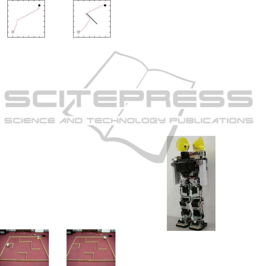
where d is the diameter of the driving wheels, and
f
x
(S(t)), f
y
(S(t)) are the x-axis increment and y-axis
increment in the local coordinates at time t, and are
defined by
f
x
(S(t)) =
4
N
A·C f
y
(S(t)) =
4
N
B·D (8)
where f
x
(S(t)) and f
y
(S(t)) are four N/4 dimen-
sional sub-space vectors of state pattern S(t), which
is shown in Fig.10. The inner products of A·B and
C·D are normalized by 4/N = 100, so f
x
(S(t)) and
f
y
(S(t)) ranges from -1 to +1.Therefore, the rotation
angle θ(S(t)) takes value from −π to π, and the mov-
ing distance L(S(t)), from 0 to
√
2πd.
4.2 Attractors for Controlling
4.2.1 Upper Layer
Figure 9: One of four embedded attractors in upper layer.
A NOVEL ADAPTIVE CONTROL VIA SIMPLE RULE(S) USING CHAOTIC DYNAMICS IN A RECURRENT
NEURAL NETWORK MODEL AND ITS HARDWARE IMPLEMENTATION
149
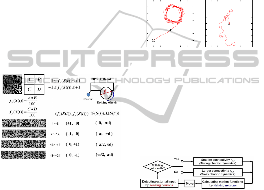
The upper layer for sensing consists of 5 in-
dependent sub-space vectors that corresponds to 5
sensors—four microphones for detecting target direc-
tion and a couple of ultrasonic sensors for detecting
obstacles, shown in Fig.9. Attractors are embedded in
the case that the direction of the maximum signal in-
tensity received by microphones is front, back, right,
or left without obstacles, respectively. As the robot
is moving, the signal intensity of four microphones
changes. Correspondingly,firing state of sensing neu-
rons in the upper layer sensitively responds to exter-
nal signal input and produce adaptive dynamics to act
driving neurons. On the other hand, if there are obsta-
cles to prevent the robot from moving forward, sens-
ing neurons corresponding to ultrasonic sensors are
activated, and cause strong chaotic dynamics in sens-
ing neurons to act driving neurons so as to enable the
robot to perform complex motions.
4.2.2 Lower Layer
Figure 10: Attractor patterns designed for motion control:
Each cyclic memory corresponds to a prototypical simple
motion.
The lower layer for driving consists of four groups
of attractor patterns, shown in Fig.10. Each attrac-
tor pattern consists of four random sub-space vectors
A,B,C and D. A and B are independent random pat-
terns. A group of specified intra-pattern structure is
given, such as A = C or −C and B = D or −D in the
present study. By the coding of motion functions,
each group of attractor pattern corresponds to one of
stationary motions in two-dimensional space.
5 CONTROL ALGORITHM
The study on RNNM tells that sufficiently large or
quite small connectivity r enables the neural network
to generate chaotic dynamics or attractor dynamics
(Nara and Davis, 1992). In quasi-layered RNNM, a
group of connectivity (r
u,u
, r
u,l
, r
l,l
) should be con-
sidered. Here, when r
l,l
is set as 60, and different
r
u,u
causes chaotic dynamics with different dynam-
ical properties. Correspondingly, by the coding of
motion functions, the robot shows weak (localized)
chaotic motions ( Fig.11(left)), or strong chaotic mo-
tions ( Fig.11(right)). On the other hand, by virtue
-0.1
0
0.1
0.2
0.3
0.4
0.5
0.6
-0.1 0 0.1 0.2 0.3 0.4 0.5 0.6
START
-8
-6
-4
-2
0
2
4
6
8
-8 -6 -4 -2 0 2 4 6 8
START
Figure 11: Examples of motion control (r
u,l
= 400 and
r
l,l
= 60): (left) larger r
u,u
= 60 generates weak chaotic
dynamics with localized property, (right) smaller r
u,u
= 20
causes strong chaotic dynamics.
of the sensitivity of chaos in quasi-RNNM, once the
best optimized connectivities are appropriately de-
termined, it will work well even when obstacle in-
formation is given to sensing neurons. However, at
the present stage, only rough target directional in-
formation is given to sensing neurons, and adaptive
switching of connectivity r
u,u
is utilized to control the
robot in two-dimensional mazes. The control algo-
rithm is shown in Fig.12. Depending on the sound
Figure 12: Control algorithm of solving 2-dimensional
mazes.
signal intensity from the target caught by four micro-
phones, sensing neurons in the upper layer sensitively
response it. Correspondingly, driving neurons in the
lower layer sensitively responds to sensing neurons
and the robot adaptively turn toward the strongest in-
tensity direction quickly due to sensitivity of chaotic
dynamics. When there are no obstacles in the range
of ultrasonic sensor, the robot moves with larger con-
nectivity r
u,u
. When there is an obstacle, it moves
chaotically with smaller connectivity r
u,u
and trys to
find detour to avoid obstacles. Several examples of
computer experiment are shown in Fig.13. In near fu-
ture, switching of connectivity r
u,u
will be replaced
ICFC 2010 - International Conference on Fuzzy Computation
150
with only sensing neurons responding to external in-
put adaptively.
-1
0
1
2
3
4
5
6
-1 0 1 2 3 4 5 6
START
TARGET
-1
0
1
2
3
4
5
6
-1 0 1 2 3 4 5 6
START
TARGET
WALL
(a) (b)
Figure 13: Examples of Computer simulation: (a) No obsta-
cle, r
uu
stays at larger one; (b) When obstacles prevent the
robot from moving forward, smaller r
uu
is used to update
the network.
6 EXPERIMENT OF HARDWARE
IMPLEMENTATION
In the present experiment, a loud speaker is set as a
target, which is emitting a specified sound signal like
calling song of a male cricket. When the robot is mov-
ing like a female cricket in two-dimensional space,
it can catch only rough directional information from
four microphones, which are attached to the front,
the back, the left and the right of the robot. Accord-
ing to the control algorithm shown in Fig.12, several
kinds of typical 2-dimensional mazes have been con-
structed. Using chaotic dynamics, the robot success-
fully avoids obstacles and reaches the target. Fig.14
shows some video snapshots of the robot solving the
above 2-dimensional maze. Now we are devoting our-
self to implement sensing neurons into the robot, and
will report them in near future.
(a) t = 0s (b) t = 408s
Figure 14: Video snapshots of the roving robot walking on a
horizontal floor where there are obstacles between the robot
and the target. Around the starting point, because the dis-
tance is a little far from the target, the robot shows chaotic
motion (a), chaotically walks for finding appropriate detour
and reaches the target (b).
7 DEVELOPING HARDWARE
IMPLEMENTATION & DEVICE
FABRICATION
Now, we briefly show our preliminary results about
the further developments based on our idea to use
functional chaos.
7.1 A Roving Humanoid Robot and an
Arm Robot Driven by Chaos
Based on our idea, we show the other examples.
One is the case that the same method of solving 2-
dimensional mazes is applied to a humanoid robot
with two legs as shown in Fig.15. This experiment is
desinged to develope our idea to 3-dimensional con-
figuration of obstacles, whereas the previous example
is to solve 2-dimensional mazes. Thus, the behaviors
necessarily include the actions not only of straddling
or to step over obstacles but also of climbing up and
down obstacles, if they would have appropriate sizes
(see Fig.16). This experment is still under going.
Figure 15: A humanoid robot used in our experiment.
The other experiment is to apply the same idea
to arm motions of animals like humanbeings or mon-
keys. However, it should be noted that we set the sit-
uation in which the robot does not have advanced vi-
sual information processing ability like manmals but
has only poor visual sensing system. The set situation
is that the sensors can detect only rough direction of
target with including uncertainty. The four infrared
light sensors are attached on the arms to realize such
ill-posed situations. (see Fig.17) At present, the ex-
periment succeed only in the case without obstacles.
(see Fig.18).
A NOVEL ADAPTIVE CONTROL VIA SIMPLE RULE(S) USING CHAOTIC DYNAMICS IN A RECURRENT
NEURAL NETWORK MODEL AND ITS HARDWARE IMPLEMENTATION
151
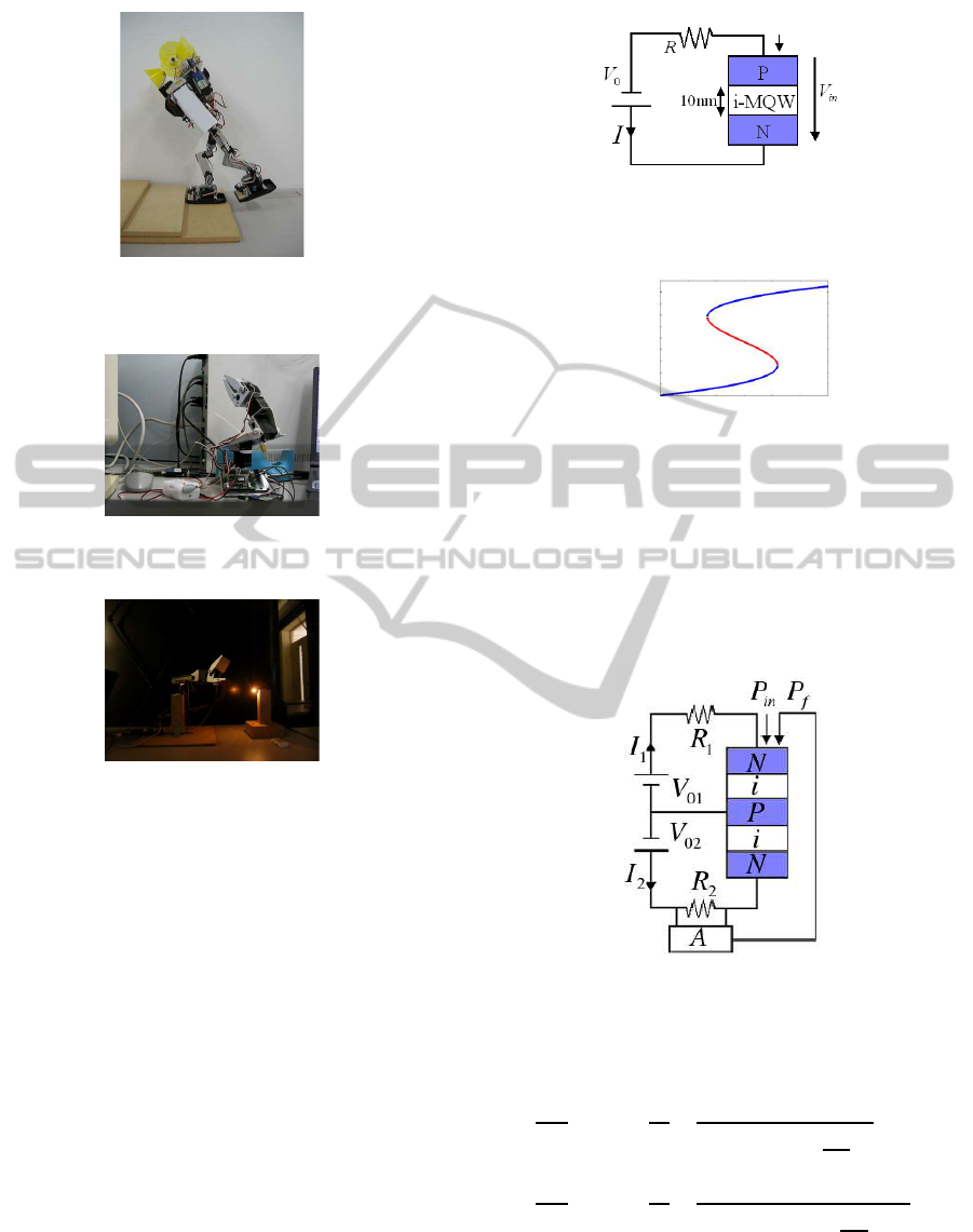
Figure 16: A humanoid robot under the action of climbing
upstairs.
Figure 17: An arm robot used in our experiment.
Figure 18: An arm robot under the action of reaching the
target.
7.2 A Pseudo-neuron Device and a
Diffusively Coupled Network of
them
In this section, we report our study about pseudo-
neuron device fabricated by Self Electro-optic Ef-
fect Device (SEED) and coupled dynamic SEED (D-
SEED).
7.2.1 Self Electro-optic Effect Device (SEED) &
Dynamic SEED
A typical single SEED composed of p-i-n semicon-
ductors is shown in Fig. 19. The primary variable
of this system is photocarrier density n which is gen-
erated by the incident optical power P
in
, where the
rate equation for photocarrier density n is given later.
The important point is that it indicates a bistable prop-
erty with respect to incident optical power as shown
in Fig.20.
in
P
Figure 19: Single SEED.
Input Power [mW]
Photocarrier Density [
×
×
×
×10
12
m
-3
]
0 0.2 0.4 0.6
0.25
0.5
Stable
Stable
Unstable
Figure 20: Bistability.
Now let us propose a pseudo-neuron device that
consists of two bistable SEED elements optically con-
nected in a series with feedback from one of them to
the power of an incident light beam (Fig. 21). We
called it ”Dynamic SEED (D-SEED)”.
Figure 21: Serially connected SEEDs with feedback.
Coupled rate equations for photocarrier density n
1
(upper) and n
2
(lower) are represented as
dn
1
dt
= −
n
1
τ
1
+
α
1
(P
in
+ P
f
)Ω
01
{ω−ξ
1
}
2
+
Ω
01
2
2
(9)
dn
2
dt
= −
n
2
τ
2
+
α
2
(P
in
+ P
f
−m
1
n
1
)Ω
02
{ω−ξ
2
}
2
+
Ω
02
2
2
(10)
ξ
i
= ω
0i
−β(V
0i
−R
i
I
i
) (i = 1,2) (11)
P
f
= AI
2
R
2
(12)
where τ, α, Ω
0
, ω, ω
0
, β, V
in
, V
0
, R, η are system pa-
rameter. Note that the primary parameter is P
in
which
ICFC 2010 - International Conference on Fuzzy Computation
152
causes many kind of bifurcation phenomena. m is ab-
sorption parameter and A is feedback gain parameter.
The rate equations show that for the upper SEED
feedback light is added to incident light, whereas the
lower SEED received the light decreased by the ab-
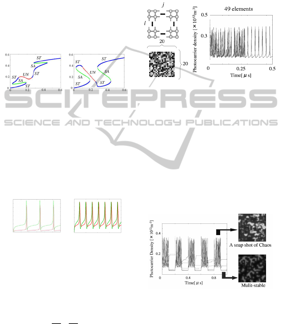
sorption in upper SEED. When we choose appropri-
ate parameter values, we can obtain various bifurca-
tion phenomena as shown in Fig. 22. Important bi-
furcations are ”Hopf bifurcation” and ”Saddle-node
bifurcation”.(Ohkawa et al., 2005)
Input Power [mW] Input Power [mW]
Photocarrier Density [
×
×
×
×10
12
m
-3
]
Photocarrier Density [
×
×
×
×10
12
m
-3
]
Figure 22: Stationary solutions of upper SEED (left) and
lower SEED (right) as a fuction of input light power P
in
.
Blue lines, green lines and red lines indicate stable ”ST”,
saddle ”SD” and unstable ”UN” respectively.
The important point of this case is that a saddle-
node bifurcation occurred on the marginal limit cy-
cle, so that, period of limit cycle becomes infinitely
long as light power approaches the saddle-node bifur-
cation point (Fig. 23). Two typical cases of oscillation
are shown in Fig. 23. Now we extend our idea to a
0.20.1
0
0.2
0.4
Photocarrier Density [×10
12
m
-3
]
Time[μs]
0.20.10
0.2
0.4
Photocarrier Density [×10
12
m
-3
]
Time[μs]
0.05
0.3
upper
lower
Figure 23: Oscillatory solutions of n
1
and n
2
for input light
power, P
in
= 0.170 (left), 0.220 (right), respectively. Note
that periods become infitely long as they approach edges
of saddle-node bifurcation points around unstable regions
(Fig. 22).
network of D-SEEDs which are diffusively coupled
in two-dimentional array. Coupled rate equations are
written include diffusion term from Eq. (13).
D
∂
2
n
∂x
2
+
∂
2
n
∂y
2
D(n
i−1, j
+ n
i+1, j
+ n
i, j−1
+ n
i, j+1
−4n
i, j
) (13)
Where (i, j) means the position of D-SEEDs in ar-
rays located in lattice points in two-dimensions, as
shown in Fig. 24 (left-up). Under cetain light power,
time-dependence of carrier density shows chaotic dy-
namics and long time behavior converge into syn-
chronaized periodic oscillation (Fig. 24 (right)). We
Figure 24: Two-dimensional square lattice D-SEEDs (left-
up), snapshot of a network state at a certain time step, where
brightness of each cell corresponds to n
i, j
and is represented
in grayscale normalized by maximum value of carrier den-
sity (left-low), and Example of time-dependence carrier
density (chaotic oscillation).
confirmed it in the numerical simulation for vari-
ous initial conditions. We obtained global spatio-
temporal chaotic dynamics if we sufficiently increase
the number of D-SEEDs. By varying light power,
we also confirmed multi-stable state. In Fig. 25,
we succeeded to obtain switching between two states,
chaotic state and multi-stable state, by varying inci-
dent light power. Now we try to apply chaos to a novel
control by adaptive switching among chaotic state,
multi-stable state and synchronized periodic state.
Figure 25: Switching between two states by varying light
power and P
in
=0.160 (Chaos) and 0.110 (Multi-stable).
7.2.2 Complex Control using Pulsed Neuron
Network
In our previous studies, The key idea is adaptive
switching between chaotic dynamics and atractor dy-
namics. Now, it is necessary to develop hardware
A NOVEL ADAPTIVE CONTROL VIA SIMPLE RULE(S) USING CHAOTIC DYNAMICS IN A RECURRENT
NEURAL NETWORK MODEL AND ITS HARDWARE IMPLEMENTATION
153
implementation of artificial neuron device. As func-
tional examples, let us pick up two cases. One is ap-
plication to motion control and the other is to mem-
ory dynamics using D-SEEDs network (pulsed neu-
ron network). In this paper, only the former is de-
scribed.
Now let us consider to solve two-dimensional
maze as an example of ill-posed problems as shown
in the previous sections. We attempt to solve maze
by adaptive switching between chaotic dynamics and
atractor dynamics with D-SEEDs network. State pat-
tern of the network is represented by 400-dimensional
state vectors, while motion in 2-dimensional space
is only two-dimensional vectors. Therefore, it is
necessary to convert 400-dimensional state to 2-
dimensional motion by coding function. We designed
3 different coding methods to prove effectiveness of
chaos which is caused various methods. Our coding
methods are introduced as follows.
(a) Adaptive switching between chaotic state and
synchronized periodic state.
(b) Adaptive switching between chaotic state and
multi-stable state.
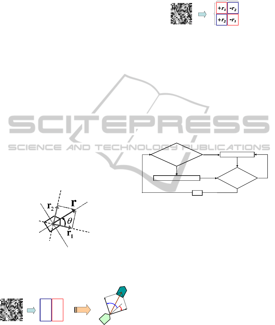
Let us consider these two cases. We calculate 2-
dimensional motion(Fig.26) from 400-dimensional
state by coding function.
Figure 26: 2-dimensional motion.
In the coding method (a), we introduce the cod-
ing but let us discard their detailed description. Next,
α
β
coding
α
β
0.5
0.5
object
Figure 27: Coding method (b)-1.
in the coding method (b), let us propose the two cod-
ing methods. One is shown in Fig.27, and the other
is shown in Fig.28, where the detailed definition of
motion increments are discarded as well.
20
20
Figure 28: Coding method (b)-2.
So it is possible to obtain 4 monotonic motions
which are almost linear motions to 4 quadrants di-
rection and chaotic motion by changing the position.
Now, we solve maze by adaptive switching between
monotonic motion and chaotic motion with a simple
control algorithm shown in Fig. 29. We assume that,
1. An object can acquire only rough direction in
which quadrant it exists.
2. The object does not have pre-knowledgeaboutob-
stacle configulation.
These context settings give an ill-posed problem.
According to the control algorithm shown in Fig. 29.
Direction of movement
Direction to target
=
=
=
=
Direction of movement
Direction to target
=
=
=
=
Direction of movement
Direction to target
=
=
=
=
Monotonic motion (multi-stable)
YES
NO
Chaotic motion (chaos)
The obstacle exists
in direction of movement
YES
Move
NO
Figure 29: Control algorithm of adaptive switching between
chaotic motion and monotonic motion.
The successful results of computer experiments were
obtained and will be reported in the conference and in
a recent paper as well.
8 CONCLUDING REMARKS
Even from the results of the present preliminary ex-
periment, we can conclude that chaotic dynamics is
useful to solve complex problems, such as mazes, not
only in computer experiments, but also in hardware
implementation of the robot systems. Although detail
consideration should be done from functional aspects,
it is at least an evidence that chaotic dynamics could
play important roles in biological systems including
brain. Therefore, we are sure that those novel func-
tional aspects of chaotic dynamics could be applied to
complex control by simple rule in systems with large
but finite degrees, and be useful to engineering ap-
plication mimicking excellent functions observed in
biological systems including brain.
ICFC 2010 - International Conference on Fuzzy Computation
154

ACKNOWLEDGEMENTS
This work has been supported by Grants-in-Aid for
Scientific Research, #19500191 in Japan Society for
the Promotion of Science and #22120509 in the Min-
istry of Education, Culture, Sports, Science & Tech-
nology.
REFERENCES
Fujii, H., Itoh, H., Aihara, K., Ichinose, N., and Tsukada,
M. (1996). Dynamical cell assembly hypothesis-
theoretical possibility of spatio-temporal coding in the
cortex. In Neural Networks. vol. 9, p. 1303.
Huber, F. and Thorson, H. (1985). Cricket auditory com-
munication. In Sci. Amer. vol. 253, pp. 60-68.
Li, Y. and Nara, S. (2008). Novel tracking function of mov-
ing target using chaotic dynamics in a recurrent neural
network model. In Cognitive Neurodynamics. vol. 2,
pp. 39 - 48.
Mikami, S. and Nara, S. (2003). Dynamical responses of
chaotic memory dynamics to weak input in a recurrent
neural network model. In Neural Computing. vol. 11,
pp. 129-136.
Nara, S. (2003). Can potentially useful dynamics to solve
complex problems emerge from constrained chaos
and/or chaotic itinerancy? In Chaos. vol. 13, pp.
1110-1121.
Nara, S. and Davis, P. (1992). Chaotic wandering and search
in a cycle memory neural network. In Progress of The-
oretical Physics. vol. 88, pp. 845-855.
Nara, S., Davis, P., Kawachi, M., and Totuji, H. (1993).
Memory search using complex dynamics in a recur-
rent neural network model. In Neural Networks. vol.
6, pp. 963-973.
Nara, S., Davis, P., Kawachi, M., and Totuji, H. (1995).
Chaotic memory dynamics in a recurrent neural net-
work with cycle memories embedded by pseudo-
inverse method. In Int. J. Bifurcation and Chaos Appl.
Sci. Eng. vol. 5, pp. 1205-1212.
Ohkawa, Y., Yamamoto, T., Nagaya, T., and Nara, S.
(2005). Dynamic behaviors of coulpled self-electro-
optic effec devices. In Appl. Phys. Lett. vol. 86, p.
111107.
Skarda, C. A. and Freeman, W. J. (1987). How brains make
chaos in order to make sense of the world. In Behav-
ioral and Brain Sciences. vol. 10, pp. 161-195.
Suemitsu, Y. and Nara, S. (2004). A solution for two-
dimensional mazes with use of chaotic dynamics in
a recurrent neural network model. In Neural Compu-
tation. vol. 16, pp. 1943-1957.
Tokuda, I., Nagashima, T., and Aihara, K. (1997). Global
bifurcation structure of chaotic neural networks and its
application to traveling salesman problems. In Neural
Networks. vol. 10, pp. 1673-1690.
Tsuda, I. (2001). Towards an interpretaion of dynamic neu-
ral activity in terms of chaotic dynamical systems. In
Behavioral and Brain Sciences. vol. 24, pp. 793-847.
A NOVEL ADAPTIVE CONTROL VIA SIMPLE RULE(S) USING CHAOTIC DYNAMICS IN A RECURRENT
NEURAL NETWORK MODEL AND ITS HARDWARE IMPLEMENTATION
155
