
A GENETIC ALGORITHM APPROACH TO A 3D HIGHWAY
ALIGNMENT DEVELOPMENT
Botan M. Ahmad AL-Hadad and Michael Mawdesley
Department of Civil Engineering, University of Nottingham,University Park, Nottingham, U.K.
Keywords: Highway alignment, Genetic algorithms, Optimization.
Abstract: This paper reports for the possibility of developing a genetic algorithm (GA) based technique model to
optimize highway alignment. It suggests a novel technique to optimize a highway alignment in a three
dimensional space. The technique considers station points to simultaneously configure both horizontal and
vertical alignment rather than considering the existing conventional principles of design which deals with
both alignments in two different stages and uses horizontal intersection points (HIP), vertical intersection
points (VIP), tangents (T), curve radii (R), deflection angles (∆), grade values (± g %), and horizontal and
vertical curve fittings to depict the horizontal and vertical alignments. The proposed method is expected to
produce a global optimal or near optimal solution and also to reduce the number of highway alignment
design elements required and consequently reduce the constraints imposed on alignment planning and
design. The results obtained have good merits and encourage further investigations for better solutions.
1 INTRODUCTION
Highway alignment development aims to connect
two terminal points at minimum possible cost
subject to the design, environmental (natural features
and air pollution), economical, social, and political
constraints. The final alignment selection will also
be affected by the public view points and decision
makers’ policy. The most common cost components
that can be considered are construction,
maintenance, location, earthwork, environmental,
and user costs. The weight of each component is
affected by the user and/or designer preferences
and/or the purpose that the alignment is built for.
All these compenents and parameters must be
considered together. However an alignment that
makes one of the parameters optimal will rarely, if
ever, make all optimal. The problem of developing
and selecting an optimum alignment is therefore
very complex but very important.
1.1 The Conventional Approach
In conventional highway design projects, highway
engineers and planners select several candidates as
alternative solutions and evaluate their suitability for
the region’s environment until coming up with the
most suitable one (Wright and Ashford, 1998).
Horizontal and vertical alignments are considered
apart from each other and the vertical one is
optimized based on the ‘best’ selected horizontal
one. This process starts by fixing several horizontal
intersection points (HIP). The number of the HIPs
may depend on the length of the highway, natural
and manmade features, and the topography. The
successive HIPs are then connected by lines thus
forming a horizontal piecewise linear trajectory.
These lines are called tangents and the deflections in
direction between successive tangents at HIPs are
called Deflection angles. Later on and in a separate
procedure horizontal circular or spiral curves are
fitted at each HIP location to form the proposed
horizontal alignment. This alignment then undergoes
an evaluation process to know whether it suits the
environment or not. The evaluation may take the
form of cost consideration, damage to environment,
and socio-economic issues subject to several design
constraints that are imposed on the alignment. This
process, through numerous iterations, is repeated
and should continue until finding the most suitable
one.
In a different process the vertical alignment is
selected using the same concept as for the horizontal
alignment. First, the elevations along the selected
horizontal alignment are determined to form the
natural ground elevation profile (NGE). Later on, to
129
Ahmad AL-Hadad B. and Mawdesley M..
A GENETIC ALGORITHM APPROACH TO A 3D HIGHWAY ALIGNMENT DEVELOPMENT.
DOI: 10.5220/0003060201290136
In Proceedings of the International Conference on Evolutionary Computation (ICEC-2010), pages 129-136
ISBN: 978-989-8425-31-7
Copyright
c
2010 SCITEPRESS (Science and Technology Publications, Lda.)

generate the alignment grade line, several vertical
intersection points (VIPs) are fixed and
interconnected successively to form a vertical
piecewise linear trajectory. The number of VIPs is
mainly affected by the variations in ground
elevations. Parabolic curves are then fitted at VIPs to
depict the vertical alignment. The vertical grade line
of the alignment is then evaluated based on the
design requirements and the amounts of earthwork
for both cut and fill sections. The process will
continue repeatedly until finding the most suitable
one.
The selection of the final alternative alignment is
accomplished by focusing on the detailed design
elements. HIPs, deflection angles, curve radii, VIPs,
tangents, grade values, and sight distances are
among the design elements of highway alignment in
3D. Most of these design elements are constrained
by standard limits described by such documents as
the Design Manual for Roads and Bridges (DMRB,
1992-2008) and AASHTO design standards
(AASHTO, 1994).
As the two processes are considered apart from
each other, the generated alignment likely represents
a local optimum rather than a global one. This
approach takes into account many design elements
and, at the same time, neglects numerous possible
solutions due to non simultaneous consideration of
both alignments. This process is also very expensive
in terms of time.
Researchers have tried to speed up the process of
highway alignment planning and design and to find
better solutions. Attempts have been done to
optimize either horizontal or vertical or both
simultaneously. Calculus of variations by Shaw and
Howard (1982), numerical analysis by Chew et al
(1989), linear programming by Easa (1988), and
genetic algorithms by Jong (1998), Fwa et al.
(2002), and Tat and Tao (2003) are some of the
techniques that have been used. The work done by
Jong (1998) has also been extended to incorporate
more cost components, GIS integration, and to
formulate the model to handle the problem as a multi
objective problem. All these can be seen in (Jong
and Schonfeld, 1999) (Jha and Schonfeld, 2000)
(Maji and Jha, 2009). It should be noted that all
these studies are based on the conventional design
principles of highway alignment design which
consider HIP, VIP, tangents, and curve fittings.
Since its introduction, despite the extreme
development in computers and highway surveying
field instruments technologies (e.g. total station),
highway engineers and planners are still using the
same convensional design approach. None of the
studies has exploited the technology development to
explore the possibility of changing some ideas
imposed on highway alignment planning and design.
A question arises here, do we still need to keep the
same planning and design approach or do we need to
change to reflect technology development? That is
the question that this study seeks to answer.
1.2 The New Approach
This study introduces a novel technique for
alignment optimization. It suggests optimizing
simultaneously the horizontal and vertical alignment
of a highway through station points. Station points
as points along the centre line of alignment, which
are defiend by their X, Y, and Z coordinates, are
used to define the alignment configuration. This
research study is inspired by the fact that any
generated alignment by whatever method will finally
consist of a series of station points and it will be
implemented on the ground depending on those
station points. Figure 1 shows the difference in
alignment generation and configuration between the
traditional and proposed method.
In this study GA, as an evolutionary adaptive
search technique (Beasley et al, 1993), is used to
perform the search. Some modifications to suit the
nature of the problem have been included (Davis
1991; Mitchell 1996).
A variety of studies have proven that GA is an
efficient tool for planning and optimization
problems. Mathews et al (1999) applied GA to land
use planning, Mawdesley et al (2002) used GA for
construction site layout in project planning, Ford
(2007) used GA for housing location planning, Jong
(1998), Fwa et al (2002), Tat and Tao (2003), and
Kang (2008) used GA for alignment optimization
problems.
2 THE MODEL FORMULATION
2.1 The Study Boundary
The study area is defined and divided into
rectangular grid cells usually produced from a GIS
model of the area under consideration. The size of
the grid cells falls within the user preferences and
depends on the desired accuracy. Each grid cell may
handle one or more than one average value. In this
study two different values are assigned to each cell.
Average land unit cost values are used for the
alignment location dependent cost calculations while
average ground elevations are used to calculate the
ICEC 2010 - International Conference on Evolutionary Computation
130
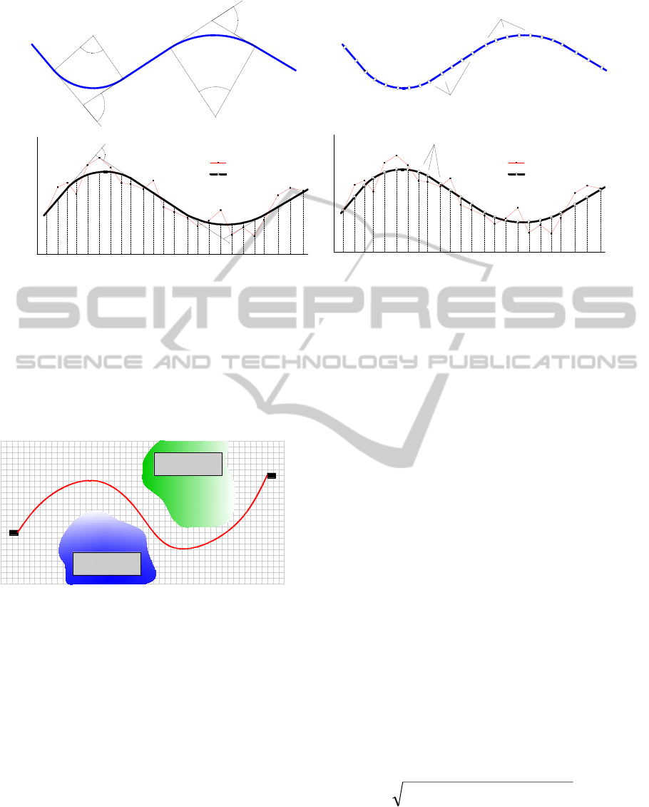
Figure 1: a & c) Horizontal and Vertical Alignment configuration with traditional method, b & d) Horizontal and Vertical
Alignment configuration using station points.
earthwork amount of cut and fill. For these purposes,
two different matrices are used for each set of data
to feed the model during the alignment development
process. Figure 2 shows a typical 2D format for a
study area:
Figure 2: Typical grid format (2D) of a study region.
2.2 The Model Cost Components
The goodness of any alignment is evaluated in terms
of cost. The lower the cost, the better will be the
solution. In general many costs could be included
and the optimum alignment should trade-off among
them. In this study, a three dimensional alignment is
modelled and tested upon few different cost
components which the experiments are based on.
These costs are related to:
1. Client or General Costs
• Length dependent cost (construction costs)
• Earthwork costs
• Location costs (environmental costs)
2. User Costs
• Fuel consumption costs
3. Geometric Design Costs
• Grade costs
• Horizontal curvature costs
• Vertical curvature costs
Other components are also possible for inclusion.
The following sections give some details for the
incorporated components.
2.2.1 Length Dependent Cost (C
Length
)
This cost directly affects the construction,
maintenance, and user costs and therefore it is
considered as one of the most influencing factors in
highway alignment optimization problems.
Highway alignment construction cost is a
function of its length. To calculate this cost, the
length of the alignment is multiplied by the unit
construction cost as:
C
Len
g
th
= L x Unit Construction Cost (1)
Where, L is the total length of the alignment. The
alignment length is a function of the x and y
coordinate of the station points (decision variables).
L =
1
0
2
1
2
1
)()(
n
i
iiii
YYXX
(1-1)
for all i = 0, 1, 2 … (n-1)
Where n is the total number of station points.
R 1
Deflection
Angle 1
PC 2
PT 2
PC 1
PT 1
HIP 1
R 2
R 2
R 1
Deflection
Angle 2
HIP 2
H Curve
H Curve
Tangent
Tangent
Tangent
Station Points
?1
?2
Station Points
( a ) ( b )
X Distances (Stations)
X Distances (Stations)
Elevations
VIP 1
g1 %
VIP 2
g2 %
g3 %
A = g2 - g1
NGE
Grade Line
Station Points
( c ) ( d )
Elevations
NGE
Grade Line
Start
End
High Unit Cost Area
(Sensitive Area
)
Proposed highway
alignment
High Unit Cost Area
(Sensitive Area)
A GENETIC ALGORITHM APPROACH TO A 3D HIGHWAY ALIGNMENT DEVELOPMENT
131

2.2.2 Location Dependent Cost (C
Location
)
This represents the costs of land acquisitions and
special requirements for construction at the locations
where the alignment passes through.
C
Location
=
p
k
k
xUCellCl
1
(2)
Where: C
Location
is the total alignment location cost;
l
k
is the length of the alignment located in a grid cell
(k) with a specific cost value; UCellC is the unit cell
cost of that cell; and p is the total number of cells
that the alignment passes through. Thus, (
∑
) where L is the length of the alignment.
2.2.3 User Costs (C
User
)
This cost represents the cost incurred by the users to
travel along the road. Here it is calculated by
multiplying the annual traffic volume (TV) by the
design life of the road (T) to give the total traffic
using the road. This in turn is multiplied by the unit
cost of the vehicle travelling unit length (UTC)
multiplied by the length of the alignment (L). Thus:
C
Use
r
= TV x T x UTC x L (3)
2.2.4 Earthwork Costs (C
EW
)
This represents the cost of earthwork in terms of cut
and fill amount. An approximate method is used to
calculate the amount of cut and fill. The difference
in elevation between the grade line and natural
ground elevation for cut (h
c
) and fill (h
f
) is
calculated and directly multiplied by the length of
that section (l
i
), width of the road (w), and unit cost
of cut and/or fill. Thus:
C
EW
l
x
h
orh
xwx
UFCorUCC
(4)
Where h
c
and h
f
is the average cut or fill depth
between station points (i+1) and (i) while l
i
is the
length of that section, and UFC or UCC is the unit
fill or cut cost.
2.2.5 Grade Violation Costs (G
Violation
)
This is a form of penalizing the solution and is
applied only when the grade of a segment between
two station points violates the maximum specified
grade. The difference in grade between the actual
calculated grade and the maximum grade is multi-
plied by a user defined cost factor.
G
|
G
G
|
xUDC
(5)
Where G
i
is the grade value between the points (i)
and (i-1) while UDC is the user defined cost factor.
2.2.6 Horizontal Curvature Violation Cost
(HC
Violation
)
Curvature of horizontal alignment is one of the
standard design requirements to ensure gradual
transition between two different directions safely at
the assigned design speed. The cost of violated
curvature according to chord definition at each
station point is considered as follow:
∑
HC
HC
then:
HC
_
HC
_
(6)
Where HC
i_existing
is the existing curvature value at
point i, HC
i_allowable
is the allowable curvature at that
point, and CVC is the curvature violation cost.
2.3 The Fitness Function
In this paper, the costs above are combined linearly
to form the total cost (C
Total
) and the aim of the
process is therefore to minimize;
C
Total
= a1.C
Traffic
+ a2.C
Location
+ a3.C
Construction
+
a4.C
Earthwork
+ a5. G
Violation
+ a6. HC
Violation
(7)
Where; a1, a2, a3, a4, a5 and a6 are weighting
factors of the individual cost components.
Other combinations of fitness function could also be
used.
3 EXPERIMENTAL SETUP
3.1 Chromosome Representation
Using the ideas of station points introduced above,
the method defines alignment through generating
station points along the centre line of the alignment.
The x, y, and z coordinates of the station points are
considered as the decision variables of the alignment
ICEC 2010 - International Conference on Evolutionary Computation
132

The chromosome map is as shown in Figure 3. It
contains the three dimensional coordinates of each
station point. The station points appear in the order
in which they occur along the length of the
alignment.
Index (i) 0 1 2 … i … … n
Individual
(j)
X
0
X
1
X
2
X
i
X
n
Y
0
Y
1
Y
2
Y
i
Y
n
Z
0
Z
1
Z
2
Z
i
Z
n
Figure 3: Chromosome representation.
3.2 Initial Population Generation
An initial population of random individuals is
generated such that:
All station points are within the study area.
X
min
≤ X
i
≤ X
max
, Y
min
≤ Y
i
≤ Y
max
,
and Z
min
≤ Z
i
≤ Z
max
where i = 1, 2, … , n-1.
The 3D components of each gene are encoded
using floating point numbers with single
precision.
The first and last points (0 and n) are fixed as the
required terminal points.
The station points are sorted in the order of their
X values (Xi ≤ Xi+1). This process is specific to
the initial population generation only.
3.3 Reproduction
3.3.1 Selection
In this study parents are selected according to their
fitness (based on ranking). The selected parents
undergo crossover and mutation to produce
offspring. The created offspring are then evaluated
by the fitness function. The fittest individuals are
merged into the population to breed in the next
generation while the bad solutions die off (Davis,
1991).
3.3.2 Crossover
In this paper a multiple random point crossover is
used to swap a segment or segments of genes
between two individuals to form two offspring. The
entire gene code (X, Y, and Z coordinates) within
the segments are swapped during this process.
3.3.3 Mutation
First, simple uniform mutation, as a standard GA
operator, is used to help the solution in evolving
over the successive generations. Different
parameters (e.g. number of individuals, number of
station points, mutation probability, number of
generations up to 100,000, and so on) have been
investigated. Moreover, different strategies have
been applied during the process. The strategies are
considered to be different mutation rates to select
different station points for mutation and dynamic
consideration of the study area. These strategies are
considered to test the level of effectiveness of the
applied method. None of these parameters and
strategies has produced a good solution.
Later, as an attempt to improve the effectiveness
of the mutation operator, the simple uniform
mutation is modified. This modified uniform
mutation (MUM) is based on that described by
Michalewicz (1999). It is adapted to associate a
number of station points with a single mutated one.
The trend of this mutation is to enhance the search,
reduce the messiness of the alignment configuration,
and to produce a smoother alignment. This operator,
as with simple uniform mutation, selects a gene
position (p) randomly and assigns a new random
value for its X, Y, and Z coordinates. Then the
operator generates two more locations (l
1
and l
2
)
provided that l
1
< p < l
2
. Then, all the genes (station
points) that locate between l
1
and p, and l
2
and p on
the other side are reallocated and put on a straight
line connecting the newly generated gene at (p) with
the selected genes at l
1
and l
2
.
4 EXPERIMENTAL RESULTS
4.1 Standard GA Tests
Figure 4 shows a typical result with simple uniform
mutation for a 2D highway alignment. A legend list
(Figure 5) is also provided to illustrate the land
feature configurations of the study region.
Figure 4: An alignment result for a horizontal highway
alignment using standard GA operators. (Land use grid
map).
A GENETIC ALGORITHM APPROACH TO A 3D HIGHWAY ALIGNMENT DEVELOPMENT
133
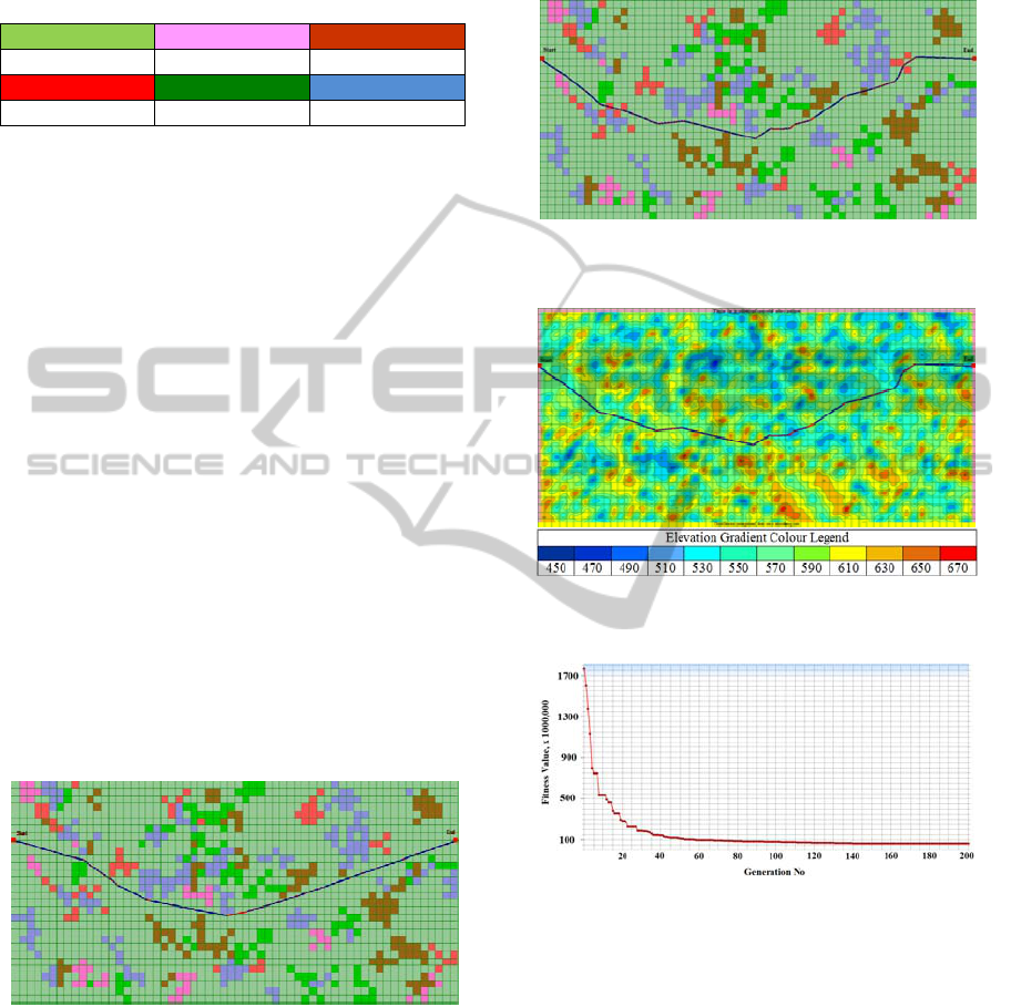
The result which obtained by this method was
not satisfactory even after 50,000 generations. The
fitness value of the final solution was 38,339,321
unit cost.
Low cost Moderate cost Normal cost
High cost Very high cost Most high cost
Figure 5: Cost colour legends of the land use grid maps.
4.2 Modified GA Tests
The modified GA formulation, which specified by
MUM as mentioned above, was also tested on a 2D
highway alignment as shown in Figure 6. The result
holds a fitness value 24,583,831 unit cost at
generation 1000. The resulting alignment is as
straight as possible, relatively smooth, and passes
through the low cost fields. The practicality of this
mutation was then tested on a 3D alignment as well.
The 3D result holds a fitness value 53,624,912 unit
cost at generation 2000. It worth to mention that this
operator, as for the 2D horizontal alignment, has the
following merits on the vertical profile:
a. It produces as low as possible earthwork costs.
b. It yields a relatively smooth alignment.
c. It tries to locate the alignment as close as possible
to the natural ground surface.
d. It tries to wind around the high and low elevation
locations to minimize cut and fill costs.
Typical results are shown in Figures 7 to 10.
Figure 6: Test result of a modified uniform mutation
(MUM) for a 2D alignment. (Land use grid map).
The two tests (2D and 3D) resulted in obtaining two
different horizontal alignment configurations
(Figures 6 & 7) due to the effect of the third
dimension (Z) on the final outcome. These
demonstrate that the horizontal and vertical
alignments are unlikely to be global optima unless
they are considered simultaneously. It should be
noted that the initial test was conducted without
considering the grade and curvature costs as they
need special techniques to handle them and these are
discussed in the succeeding sections.
Figure 7: Horizontal alignment test result of MUM for a
3D highway alignment. (Land use grid map).
Figure 8: Horizontal alignment result of MUM for a 3D
alignment on contour map.
Figure 9: Fitness graph. (Note: only the substantial
improvements over 200 generations are shown).
However, as is clear in the results, the modified
uniform mutation (MUM) method still keeps some
sharp bends (horizontally and vertically) throughout
the length of the alignment. These sharp bends are
expected from such a mutation method.
Furthermore, the vertical one possesses some
grades (upwards and downwards) which are greater
than the maximum permitted one. These alignment
criteria cannot be improved unless specific
algorithm techniques are developed and associated
with the search process. This needs to be considered
as constraints according to the geometric design and
safety requirements of the highway.
ICEC 2010 - International Conference on Evolutionary Computation
134
Figure 10: Vertical alignment profile result (grade line elevations) of MUM for a 3D highway alignment.
4.3 Grade and curvature Constraint
Handling Technique Tests
Three different algorithms are developed to handle
curvature for the horizontal alignment, curvature and
gradient for the vertical alignment. Penalty and
repair techniques are considered to look after the
point locations along the alignment that violate the
allowable horizontal curvature limits. Penalty is used
for maximum gradient violation while repair
technique is applied for vertical curvature violation.
The formulations of these techniques are based on
standard design requirements for both geometric
design and safety. These techniques are individually
applied to each single station point or location where
the violations exist.
Different experiments have been carried out to
test the effect of each technique separately and
simultaneously. The test results show that the
resulting solutions are improved significantly as
shown in Figure 11 to 13. The results show that the
solution is good with no or very few gradient and
curvature violations.
Figure 11: Horizontal alignment result for a 3D alignment
evolved with curvature and grading constraint handling.
(Land use grid map).
Figure 12: Horizontal alignment result for a 3D alignment
evolved with curvature and grading constraint handling.
(Contour map).
5 CONCLUSIONS
A three dimensional highway alignment
optimization model based on a genetic algorithm has
been developed. A new technique has been
introduced to define the alignment configuration.
Station points along the centre line of the alignment
have been used to generate alignments of different
configurations. Specific genetic algorithm operators
and constraint handling techniques were tested and
the results indicate that the method holds promises.
The results also show that the station point
technique is promising if it is assisted by constraint
handling algorithms to produce better solutions. It is
concluded that the constraint handling techniques
assisted in the improvement of the alignment
curvature characteristics and the reduction or
prohibition of the gradient violations.
However, the results show that further
developments and further investigations are required
to verify generating more realistic alignments. More
specific GA operators and further modifier and
constraint handling techniques will be investigated.
Moreover, the model needs to be tested on different
worlds and the model parameters need to be
determined and verified for applicability in real
world application problems.
A GENETIC ALGORITHM APPROACH TO A 3D HIGHWAY ALIGNMENT DEVELOPMENT
135
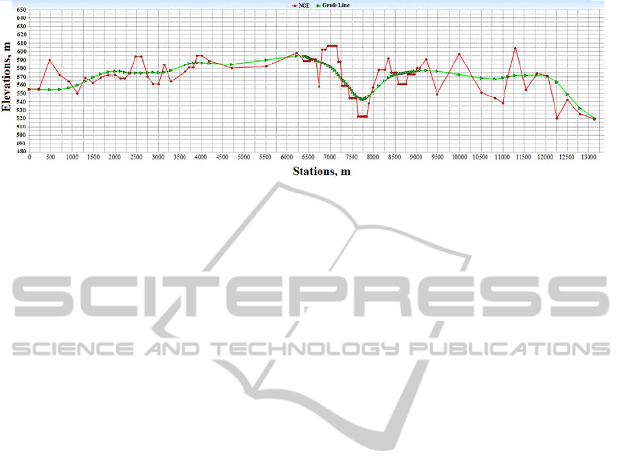
Figure 13: Vertical alignment profile for a 3D highway alignment evolved with curvature and grading constraint handling.
REFERENCES
American Association of State Highway and
Transportation Officials, 1994. USA.
Beasley, D., Bull, D. R., and Martin, R. R., 1993. An
Overview of Genetic Algorithms: Part 1
Fundamentals, University of Computing, 15(2), 58-69.
Chew, E. P., Goh, C. J., and Fwa, T. F., 1989.
Simultaneous Optimization of Horizontal and Vertical
Alignments of Highways, Transportation research,
Part B, 23(5), 315-329.
Davis, L., 1991. Handbook of Genetic Algorithms, Van
Nostrand Reinhold, New York, USA.
Design Manual for Roads and Bridges, (1992-2008). The
Highways Agency, UK.
Ford, M., 2007. A Genetic Algorithm Based Decision
Support System for the Sustainable Location of
development Allocations, Ph.D. Thesis, University of
Nottingham, UK.
Fwa, T. F., Chan, W. T. and Sim, Y. P., 2002. Optimal
Vertical Alignment Analysis for Highway Design,
Journal of Transportation Engineering, Vol. 128, No.
5, pp. 395 – 402.
Jha, M. K. and Schonfeld, P., 2000. Integrating Genetic
Algorithms and Geographic Information System to
Optimize Highway Alignments, Transportation
Research Record, 1719, 233-240.
Jong, J. C., 1998. Optimizing Highway Alignments with
Genetic Algorithms, Ph.D. dissertation, University of
Maryland, College Park, USA.
Jong, J. C. and Schonfeld, P., 1999. Cost Functions for
Optimizing Highway Alignments, Transportation Re-
search Record, 1659, 58-67.
Maji, A. and Jha, M. K., 2009. Multi-Objective Highway
Alignment Optimization Using A Genetic Algorithm,
Journal of Advanced Transportation, 43 (4), 481-504.
Mathews, K. B., Craws, S., Mackenzie, I., Elder, S. and
Sibbald, A. R., 1999. Applying Genetic Algorithms to
Land Use Planning. In: Proceedings of the 18
th
Workshop of the UK Planning and Scheduling Spatial
Interest Group, 1999, University of Salford, UK.
Mawdesley, M. J., AL-Jibouri, S. H. & Yang, H., 2002.
Genetic Algorithms for Construction Site Layout in
Project Planning, Journal of Construction Engineering
and Management, 128 (5), 418-426.
Michalewicz, Z., 1999. Genetic Algorithms + Data
Structures = Evolution Programs, Springer-Verlag,
USA.
Mitchell, M., 1996. An Introduction to Genetic
Algorithms, The MIT Press, USA.
Shaw, J. F. B. and Howard, B. E., 1982. Expressway
Route Optimization by OCP, Journal of
Transportation Engineering, ASCE, 108(3), 227-243.
Tat, C. W. & Tao, F., 2003. Using GIS and Genetic
Algorithms in Highway Alignment Optimization,
Intelligent Transportation System, 2, 1563-1567.
Wright, P. H. & Ashford, N. J., 1998. Transportation
Engineering: Planning and Design, John Wiley and
Sons, USA.
ICEC 2010 - International Conference on Evolutionary Computation
136
