
AUTOMATIC GAIN CONTROL NETWORKS FOR
MULTIDIMENTIONAL VISUAL ADAPTATION
S. Furman and Y. Y. Zeevi
Faculty of Electrical Engineering, Technion, Haifa 32000, Israel
Keywords: Non-linear Recurrent NN, Visual Adaptation, AGC, HVS, Size, Depth, Curvature, Enhancement.
Abstract: Processing and analysis of images are implemented in the multidimensional space of visual information
representation. This space includes the well investigated dimensions of intensity, color and spatio-temporal
frequency. There are, however, additional less investigated dimensions such as curvature, size and depth
(for example - from binocular disparity). Along these dimensions, the human visual system (HVS) enhances
and emphasizes important image attributes by adaptation and nonlinear filtering. It is interesting and
possible to emulate the visual system processing of images along these dimensions, in order to achieve
intelligent image processing and computer vision. Sparsely connected, recurrent adaptive sensory neural
network (NN), incorporating non-linear interactions in the feedback loops, are presented. Such generic NN
exhibit Automatic Gain Control (AGC) model of processing along the visual dimensions. The results are
compared with those of psychophysical experiments exhibiting good reproduction of visual illusions.
1 INTRODUCTION
The perceived image is quite different from the
original image projected onto the retina. Some of the
image features are enhanced, while others are being
adapted to or even ignored. Some features are of
great importance, while other are barely noticed.
Understanding the organization and functioning
of visual systems is obviously of great interest and
importance to brain scientists and engineers because
of its potential use in the design of technological
systems. By matching image presentations (or
storage) with the known performance of the visual
system, more meaningful and efficient
communication can be achieved. After all, most
information generated for human use, is
communicated with the human observer via the
visual system as the final receiver. In yet another
way, image processing modelled after the visual
system may prove to be important in machine vision.
And of course, if visual prosthetics are to become a
workable reality, this understanding is essential.
Each cone in the central fovea is connected to
about 4000 cortical neurons (Zeevi & Kronauer
1985). The challenge is to determine what the 4000
or so different processes are, and then how they are
ordered in the tissue volume. Orientation and ocular
dominance (OD) (Hubel & Wiesel 1979) can
account for 40 different processing units (20
different orientations for each ocular projection).
This leaves an unexplained factor of 4000/40=100!
There are several candidates for the remaining
functions, such as color, intensity, texture, curvature,
range of field sizes and binocular disparity (for
depth perception).
Gibson (1937) had claimed that adaptation and
negative after-effect are to be conceived as a process
of adjustment and readjustment of the physical-
phenomenal correspondence of a certain type of
sensory dimension, under the influence of a
tendency for sensory activity to become normal,
standard or neutral. He noticed that this similarity
cuts across the sensory modalities of our world,
including pressure, size, distance, temperature,
brightness, curvature (convex-concave), etc.
Zeevi & Mangoubi (1978) showed that
Adaptation plays an important role in the
suppression of quantal and receptor internal noise.
Wainwright (1999) proposed that visual adaptation
in orientation, spatial frequency, and motion can be
understood from the perspective of optimal
information transmission.
Automatic Gain Control (AGC) has been widely
used to account for intensity adaptation (Shefer
1979) contrast adaptation in the primary visual
163
Furman S. and Zeevi Y..
AUTOMATIC GAIN CONTROL NETWORKS FOR MULTIDIMENTIONAL VISUAL ADAPTATION.
DOI: 10.5220/0003061901630175
In Proceedings of the International Conference on Fuzzy Computation and 2nd International Conference on Neural Computation (ICNC-2010), pages
163-175
ISBN: 978-989-8425-32-4
Copyright
c
2010 SCITEPRESS (Science and Technology Publications, Lda.)
cortex (Weltsch-Cohen 2002), contrast adaptation
for “cyclopean” image (Ding & G. Sperling 2006),
contrast adaptation for motion detection (Lu &
George Sperling 1996) chromatic adaptation (Du
Croz & Rushton 1966) and (Krauskopf & Mollon
1971), and sound adaptation (Schwartz & Simoncelli
2001). It is, therefore, natural and tempting to
implement AGC NN which incorporates some other,
less investigated dimensions of adaptation, such as
size, depth and curvature in processing of images.
Likewise, such an investigation may facilitate our
understanding of how adaptation along these
dimensions takes place in the visual system (or other
sensory modalities for this matter).
The purpose of this study is to analyze adaptation
along these image dimensions and process these
image attributes by means of the AGC model in
order to mimic the human visual system (HVS), and
to propose a unified model for biological sensory
processing. Likewise, the AGC mechanism
considered in the context of visual systems
(biological and ANN-based alike), can be also
implemented in advanced image processing
algorithms that highlight various image structures
and feature. The performance of the proposed AGC
NN is tested by computer simulations, using Matlab,
for each dimension separately.
2 VISUAL AGC MODEL
The proposed AGC model of visual adaptation is
based on the original work of Shefer (1979), and on
the subsequent development of the adaptive
sensitivity camera that mimics the eye (Ginosar et al.
1992) and (Zeevi et al. 1995). The model has been
motivated by the structure and function of the eye
and, in particular, by its high spatio-temporal
sensitivity to small changes in intensity
accomplished over extremely wide dynamic range.
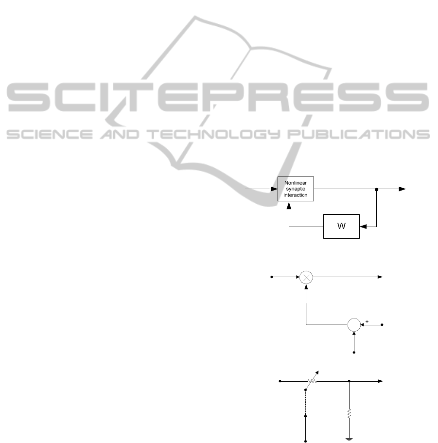
According to this nonlinear adaptation model, the
output of a cell in location “
i ” is adjusted by
subtracting from its input a nonlinear function of its
input and a weighted sum of the outputs, fed back
into the nonlinear synaptic operator (Fig. 1):
(, )T
iiii
rssf
α
=⋅−
,
(1)
where
i
r is the output,
i
s
is the input, W is a
feedback operator (matrix),
i
f
is the feedback (see
Eq. 2),
α
is a constant and T is a nonlinear function.
The crucial ingredient of this AGC model is the
nonlinearity within the feedback loop (i.e. the
function T). This is a fundamental extension of the
lateral inhibition recurrent NN into the nonlinear
regime, presumed to be mediated biologically by the
retinal interplexiform cells and/or similar structures
in other sensory neural networks, such as the
synaptic depression (Abbott et al. 1997). It is
important to note that qualitatively T may assume a
wide range of nonlinear functions and, yet, the
neural feedback loop in which such nonlinear
synaptic interactions are embedded will exhibit
functional AGC.
In a specific embodiment of this general
conceptual model, the nonlinearly component is a
multiplier (Fig. 2a). The model is then comprised of
a series of static multipliers, one for each foveal
receptor channel that multiply the input of the
channel with the output of the feedback. The
feedback is calculated by subtracting the output of
the operator "W" from a constant value. The
operator "W" is an averaging operator (in space).
The analytic domain of the model, in which we
will be interested, is the upper right handed quarter
of the multiplier. It is possible to choose the operator
"W" so the model will operate at the analytic domain
for an input i changing in a defined known range.
We will assume that this is the case.
i
r
i
s
i
f
Figure 1: AGC model.
(a)
(
b
)
Σ
i
r
i
s
α
i
f
i
r
i
f
i
s
Figure 2: Gain control device. (a) Schematic drawing; (b)
Hypothetic explicit implementation.
The presented AGC NN necessitates the existence of
ICFC 2010 - International Conference on Fuzzy Computation
164

controlled gain device. One option for such a device
is shown in Fig. 2b. Bruckstein and Zeevi (1979)
showed that the gain control of Fig. 2 can be
implemented by a neural coding scheme with
threshold control.
Each of the functions of the model is of an image
dimension (curvature, size and depth). The feedback
is obtained by:
ijij
j
f
wr=
∑
.
(2)
Therefore the AGC model output is given by:
()
ii jij
j
rs wr
α
=−
∑
.
(3)
The function of the feedback is to position
symmetrically the oparting curve around the
operating point. W can be chosen as exponent,
gaussian, triangle, rectangular or any other
symmetric kernel without effect on the main
characters of the model.
The model has a unique solution for
1
0max{}
ii
i
W
s i and s
S
≥∀ < ,
(4)
where
W
S is:
Wji
j
Sw=
∑
.
(5)
ii
i
rr
ε
−<
∑
%
i
s
ii
s
r→
ii
rr→
%
ji j i
j
wr f→
∑
(1 )
iii
s
fr−→
i
r
Figure 3: Flow chart for calcuating the visual AGC
response to some arbitrary input.
2.1 Small Signal Analysis
Although we are concerned with “large signal”
behaviour of the visual AGC, it is still useful to
perform small signal analysis of the model. For that
we assume that both the output and the input of the
model are composed of a ‘local DC’,
s
C (where
local is defined on the scale of effective W)
modulated by a small AC signal component:
isi
SCs
=
+ ,
(6)
0
i
i
s
=
∑
,
(7)
iri
RCr
=
+ ,
(8)
0
i
i
r
=
∑
.
(9)
For simplicity, we assume also that W is a
rectangular function. Under these assumptions, (2)
yields:
ijijr
j
f
wR C
=
=
∑
,
(10)
substituting (6),(7),(8),(9) and (10) in (3), we get:
;
11
s
ii r
s
s
C
rs C
CC
α
α
⋅
==
++
.
(11)
Equation (11) expresses a sigmoidal function, which
is closely related to Weber law. The latter implies
that the system gain is inversely proportional to the
input’s average.
Weber law is characteristic for many sensory
modalities, including weight, vision and sound.
0 10 20 30 40 50 60 70 80
0.1
0.2
0.3
0.4
0.5
0.6
0.7
0.8
x
input step
output
Figure 4: AGC model step response.
2.2 Simulation Method
In its discrete form, Eq. (3) exhibits the complexity
of a manybody problem. To obtain a closed form
solution for some arbitrary input is a major
challenge, not yet dealt with. Therefore, we use a
numeric solution of an iterative process. In the
discrete final case, the solution is unique if the
process converges (Shefer 1979). Fig. 3 presents the
flow chart of the algorithm for numeric solution of
the AGC model.
AUTOMATIC GAIN CONTROL NETWORKS FOR MULTIDIMENTIONAL VISUAL ADAPTATION
165
0
20
40
60
80
0
1
2
3
0.1
0.2
0.3
0.4
0.5
x
I(x)
Figure 5: Ramp responses for various input slopes.
2.3 Step Response for AGC Model
Fig. 4 depicts step response of the non-linear AGC
model, superimposed on the step. This example
highlights the main characteristics of the model:
The adapted response to a locally-constant input
is being decreased, while high values are more
affected than lower values. This is, in a way,
compression of a wide dynamic range of the
input.
An edge enhancement – the relative contrast is
increased. This is caused by the overshoot and
undershoot of the model response. Note that due
to the nonlinearity of the model, the overshoot is
stronger than the undershoot. Fig. 5 shows
another nonlinear effect – the
overshoot/undershoot are depended on the slop
of the input step. The response is stronger for
steeper slopes. When the input represents
intensity, this phenomenon is the well known
"Mach Bands" (Ratliff 1965).
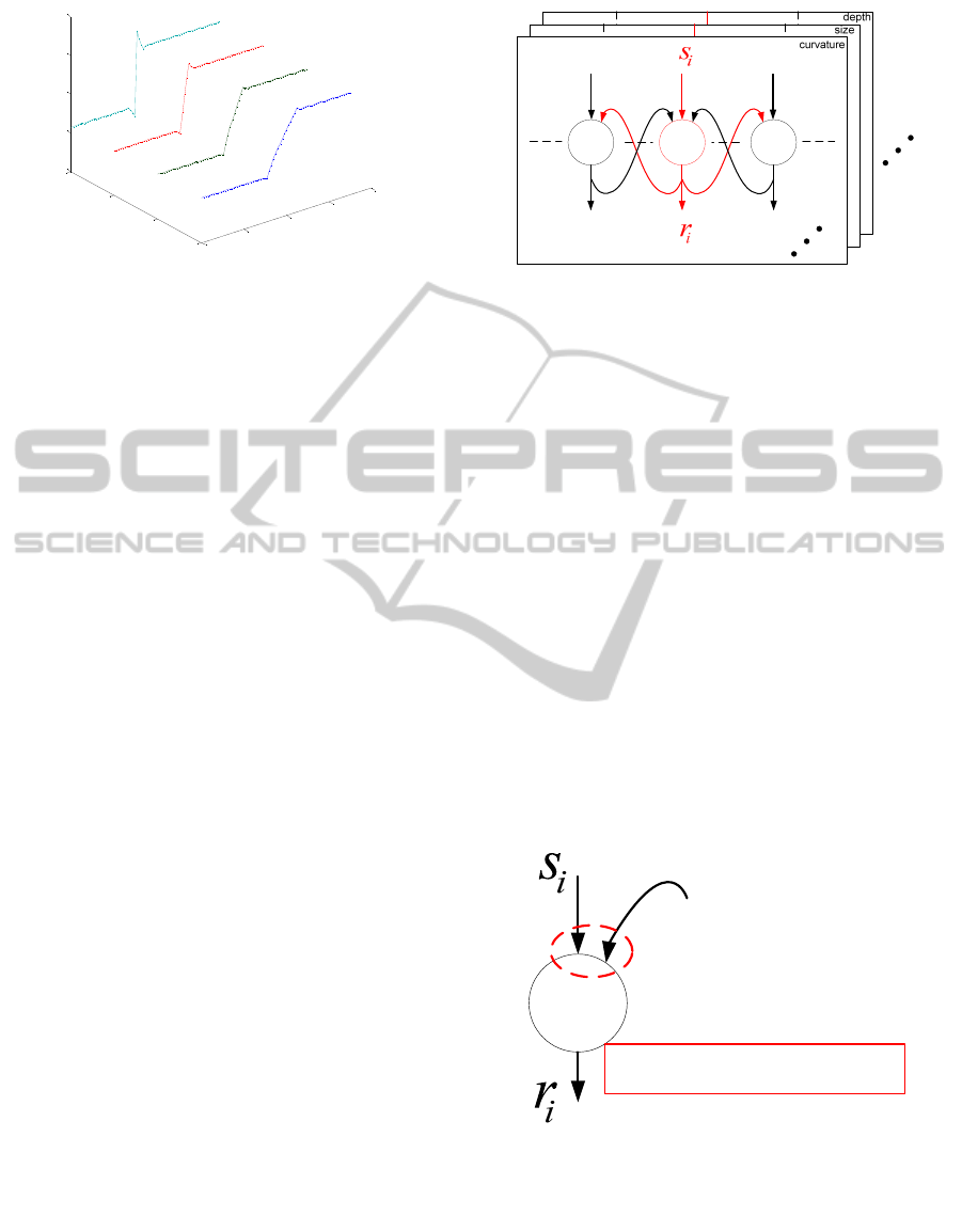
2.4 AGC NN
The adaptive, non-linear, recurrent NN which
exhibits multidimensional AGC characteristics
constitutes in its functional complexity a case of a
many-body problem. Yet, due to the local
characteristics of W in the case of visual information
processing, the network is sparsely connected and
the implementation is simple and efficient with only
one layer of a recurrent neural network (RNN). Fig.
6 depicts a schematic structure of such a RNN. One
should keep in mind that each neuron represents a
nonlinear function, as shown in Fig. 7. This is
biologically feasible (as discussed above). It can be
implemented in NN by other types of nonlinearities
and architechtural embodiments.
i
N
l
N
m
N
mi m
wr
li l
wr
m
r
l
r
m
s
l
s
Figure 6: AGC NN.
3 BACKGROUND
3.1 Localness and Parallelism
A key fact regarding the structural-functional
organization of the HVS (which support our AGC
NN model) is that processing along the image
dimensions of size, curvature, depth and/or other
dimensions is performed locally and in parallel over
the entire image (Hochstein & Ahissar 2002). These
image dimensions are believed to be part of the
"Elementary Features" (Cavanagh et al. 1990),
(Wolfe et al. 2003) of the image representation in
the HVS. In this case, the image is decomposed
along a number of dimensions and into a number of
separable components, and some specific cells
represent that local information (a concept
introduced by Hubel and Wiesel (1968) within the
context of retinotopic representation).
ijij
j
f
wr
=
∑
(, )
iiii
rssf
α
=
⋅−T
Figure 7: Nonlinear function of each neuron.
This concept had been tested in many
psychophysical experiments such as “pop-ups”. In
these experiments, there is a target with a unique
feature which is not shared by the distractors.
If the feature is coded early in the visual processing
and is performed locally and in parallel, the target
ICFC 2010 - International Conference on Fuzzy Computation
166
tends to “pop-up” from the distractors with little
effect of the number of distractors. The features may
either be discrete and categorical elements (e.g.,
terminators) that can be only present or absent, or
they may be values on a continuous dimension that
activate nonoverlapping populations of functional
detectors and that, therefore, also mediate
categorical discriminations. Treisman & Gormican
(1988) showed that such "pop-up"s are asymmetric
in that some features are detected more easily when
they are present rather than when they are absent.
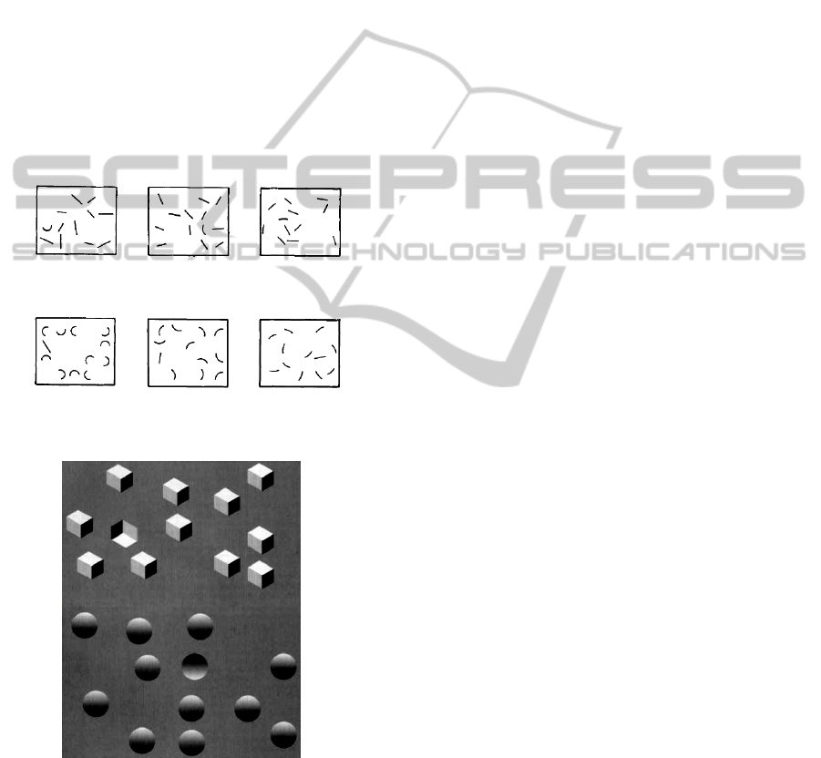
Fig. 8 (adopted form (Treisman & Gormican 1988))
presents an example of such experiment for a target
defined by curvature, while Fig. 9 presents an
example of such experiment for target defined by
depth cues (See Enns & Rensink (1990a), (1990b)).
Thus, we may conclude that size, curvature and
depth are processed locally and in parallel.
Figure 8: Examples of displays testing search for targets
defined by curvature or ‘straightness’.
Figure 9: Two examples of display, testing search for
targets defined by depth cues.
3.2 Adaptation and Feature Detectors
It is well known that prolonged inspection of a
curved line causes adaptation to curvature (e.g. the
curvature after-effect (Gibson 1937) and (Coltheart
1971)). Such after-effects are believed to reflect a
change in the sensitivity of neurons that encode the
adapted feature and, thus, imply the existence of
neurons that act as detectors of that feature
(Hancock & Peirce 2008).
Indeed, most of the investigators agree that
curvature detectors are present along the early stages
of the visual pathway (Riggs 1973), (Stromeyer &
Riggs 1974). Some investigators even showed how
such curvature calculations can be achieved by
convolution with certain reasonable receptive fields
of neural cells (Koenderink & Doorn 1987),
(Dobbins et al. 1987).
Sutherland (1968) concluded that many species
have the capacity to classify a shape as the same
shape regardless of changes in size, at least over a
considerable range, and that this capacity is innate.
This ability can be addressed as irrelevance of the
DC component of the size information (adaptation)
and relevance of changes only.
Blakemore and Campbell (1969) suggested that
the human visual system may possess neurons
selectively sensitive to size. They also suggested that
this neural system may play an essential preliminary
role in the recognition of complex images. Carey et
al (1996) suggested that size, motion and orientation
measures are processed in parallel by the dorsal
stream mechanisms.
The visual system perceives depth based on
several cues such as stereoscopic views, motion-
parallax, object size, object translation and rotation
(Bruno & Cutting 1988), (Dijkstra et al. 1995),
(Rogers & Graham 1979), (Bradshaw & Rogers
1996) and (Bradshaw et al. 2000). Hubel and Wiesel
(1962), (1970) have identified the cells that are
involved in depth information representation from
stereoscopic vision (“complex cells”). Inui et al
(2000) have discovered that an area involved in
monocular depth processing in the bilateral
occipitotemporal region.
It, therefore, seems reasonable to assume that
curvature, size and depth information are calculated
over the entire image (in parallel), wherein each of
the cells contains the feature information of a
specific location - each cell represents the feature
information of a specific part of the image and
together they create a projection of the image into a
specific image dimension, where the location of the
cells matches the location of the feature in the
image. Based on this reasoning, it is natural to use
AGC NN in processing of these image dimensions
in vision.
AUTOMATIC GAIN CONTROL NETWORKS FOR MULTIDIMENTIONAL VISUAL ADAPTATION
167
3.3 Overview of Differential Geometry
It is useful to review a few elementary notions of
differential geometry to establish the context in
which the curvature processing is formulated. The
review is focused on curves in the plane, although
generalizations to higher dimensional curves exist.
Let
I
be an interval in one-dimensional
Euclidian space
1
E . A curve C is defined as a
continuous mapping
2
:
x
IE→
from the interval to
the plane where
()
12
((), ())xxx
λ
λλ
=
,
(12)
with
I
λ
∈
being a parameter running along the
curve, and
12
,
x
x
are continuous functions of
λ
. The
curve is said to have order of continuity k, denoted
by
k
C
, where all derivatives up to and including the
k
th
derivative of
1
x
and
2
x
are continuous. A curve
may be reparameterized in terms of its arc length s,
equivalent to a particle travelling at constant unit
velocity along the curve. In this case, the tangent
vectors are unit length vectors:
()
12
' ( ) ( '( ), '( ))
x
sts xsxs==
,
(13)
where
()sf
λ
=
is a reparameterization of the curve,
and
'1x =
. The interesting aspect of the tangent is
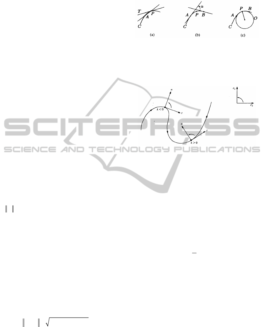
its orientation. The geometric interpretation of the
tangent to a curve is depicted in Fig. 10(a). Letting P
be a point on a curve, and A a neighboring point, the
tangent T at P is the limit of the line AP as A
approaches P along the curve. The tangent yields
the orientation of a curve at a point. Taking the
second derivative with respect to s everywhere along
C, we obtain
(
)
12
'' ( ''( ), ''( ))
x
sxsxs=
,
(14)
where the vector
''( )
x
s
is normal to the vector
'( )
x
s
and the magnitude of
''( )
x
s
is the curvature of C:
()
22
12
'' '' ( ) '' ( )
x
sxsxs
κ
== +
.
(15)
Curvature is a measure of the rate of change of
orientation per unit arc length. The geometric
interpretation for the curvature is depicted in Fig.
10(b). Let P be a point on a curve, T the tangent at
that point, and A a neighboring point on the curve.
Figure 10: (a) Tangent T is the limit of segment PA as A
approaches P along C. (b) The curvature
κ
of C at P is the
limit of the ratio
α
/AB as A and B approach P
independently along C. (c) The osculating circle 0 at P is
the limit of the circle that passes through A, P, and B, as A
and B approach P.
Figure 11: Signed curvature.
Let
α
denote the angle between the line AP and T,
and AB the arc length between A and B. The
curvature
κ
at P is the limit of the ratio
α
/AB as A
approaches P along the curve. Related to this
interpretation of curvature is the osculating circle.
Referring to Fig. 10(c), let A, P, and B be three
neighboring points on a curve, and let U be a circle
through these points. As A and B independently
approach P along the curve, the circle O converges
towards a limit, whose radius is precisely the inverse
of the curvature
κ
at P.
1
R
κ
=
.
(16)
Since the curve is a plane curve (that is,
()
x
I is
contained in a plane), it is possible to associate a
sign with the curvature
κ
. To this end, let
{
}
12
,ee
be
the natural basis of
2
R
,
and define the normal
vector
(),ns s I
∈
, by requiring the basis and might
be either positive or negative. It is clear that |
κ
|
agrees with the previous definition and that
κ
changes sign when we change either the
orientation of
x
or the orientation of
2
R (see Fig. 11).
In this work, we use the signed curvature notation.
The signed curvature indicates the direction along
which the unit tangent vector rotates as a function of
the parameter along the curve.
ICFC 2010 - International Conference on Fuzzy Computation
168
{
}
(), ()ts ns
to have the same orientation as the
basis
{
}
12
,ee
. The signed curvature
κ
is then defined
(instead of (15)) by
'( )ts n
κ
= ,
(17)
If the unit tangent rotates counter clockwise, then
0
κ
>
. If it rotates clockwise, then
0
κ
<
.
The signed curvature depends on the particular
parameterization chosen for a curve.
4 PSYCHOPHYSICAL
EXPERIMENTS
For illustrative purpose, two psychophysical
experiments are presented as an example. The first is
for size contrast effect (the Ebbinghaus illusion).
The second is for depth contrast effect. The AGC
model reproduces the illusions.
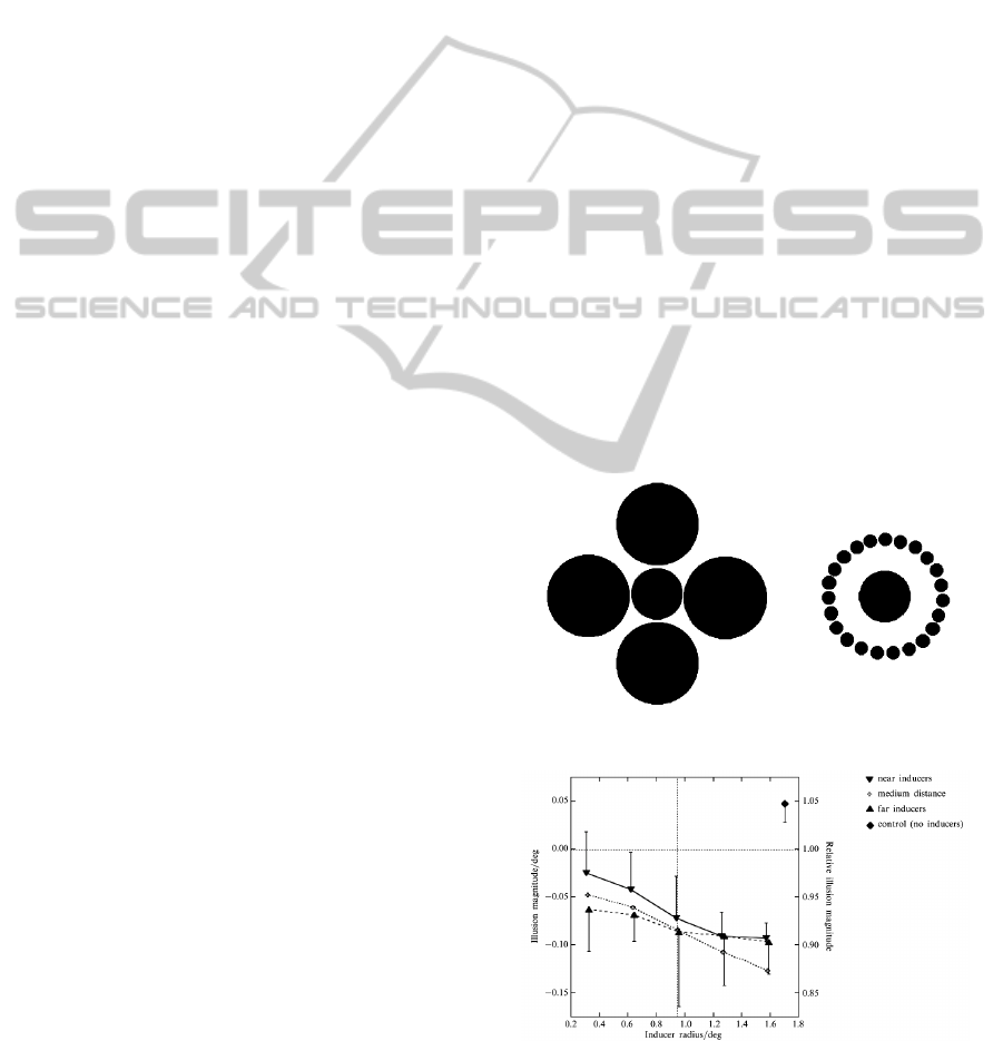
4.1 Size Contrast
The Ebbinghaus illusion is commonly used as an
example of a simple size-contrast effect. In this
illusion, the apparent size of a central target is
changed by a ring of surrounding inducers. Fig. 12
illustrates its most popular form, as it most often
appears in general textbooks. In this form, it is
typically used to illustrate a simple size-contrast
effect, in which large inducers make the target
appear smaller whilst small inducers make it
appear larger.
Roberts et al (2005) have further investigated the
above effect and concluded that it probably arises
from a number of factors that are:
The relative size and number of the inducers
(comparing to the target): For a given distance
between the target and the inducers, the
magnitude of the Ebbinghaus illusion is
governed by the relative size and number of the
inducers
The distance between the central target and the
inducers: For a given number and size of
inducers, the magnitude of the Ebbinghaus
illusion is governed by the distance between the
central target and the inducers.
The completeness of the inducing annulus:
Keeping the number of the inducers constant,
and changing their size (or distant), provides a
change in the completeness of the inducing
annulus. This confounding effect can be
removed (the inducing annulus can be kept
constant) by changing also the number of the
inducers.
The authors performed several experiments, and the
main findings were:
4.1.1 Experiment 1
Varying the relative size of the inducers in the
Ebbinghaus illusion produces changes in the
apparent size of the target, consistent with a size-
contrast effect. Increasing inducer distance causes a
decrease in apparent target size irrespective of
inducer size. [Distance is measured from the centre
of the target to the centre of the inducers.]
Fig. 13 shows, separately for each inducer
distance, the average illusion magnitude, as a
function of inducer radius. Based on these results,
the authors concluded that “inducers generally
reduce apparent target size and that small inducers
are simply less effectual in doing this”, and that
“Inducer distance also has an effect, so that the
reduction in target size tends to be more pronounced
at greater distances”.
To summarize, the apparent size of the target is
reduced more efficiently when the inducers get
bigger and at greater distances.
Figure 12: The Ebbinghaus illusion.
Figure 13: Results of experiment 1 from (Roberts et al.
2005).
AUTOMATIC GAIN CONTROL NETWORKS FOR MULTIDIMENTIONAL VISUAL ADAPTATION
169
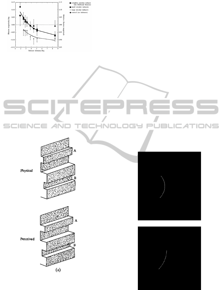
Figure 14: Results of experiment 3 from (Roberts et al.
2005).
4.1.2 Experiment 3
Here, The authors kept the inducing annulus and
inducer size constant and study the effect of inducer
distance. The results are given in Fig. 14. The
authors conclude that the data can be modelled by
the equation
exp( / )ab xc+− and that the effect is
governed mainly by two terms – inducers distance
from the target (which described by decaying
exponential), and by the inducers size which
modulate this function.
Figure 15: Bar A appeared to lie in front of bar B,
although are physically at the same depth.
4.2 Depth Contrast
Graham and Rogers (1982) have shown depth-
contrast effect perceived from motion parallax and
stereoscopic information. Their results are shown in
Fig. 15. The perceived depth is affected by the
surrounding, and so, even though bar A and bar B
are at the same physical depth, they are perceived as
though bar A is in front of bar B.
5 SIMULATION RESULTS
We assume that the features information is
represented, and we are not concerned with the issue
of how this information was acquired. This
assumption is quite valid because many techniques
of depth/size/curves (and therefore – their curvature)
estimation are available today. An example for such
technique for curves is presented by Parent &
Zucker (1989) and Zucker et al (1988).
In order to simulate a feature processing and see
its effect on a human observer, a tool (Matlab
function) that draws image corresponding to its
feature information input was created. The image
was then drawn according to its original feature
information, and according to its processed feature
information.
original curve
original curve filtered with AGC
Figure 16: AGC of constant curvature.
ICFC 2010 - International Conference on Fuzzy Computation
170
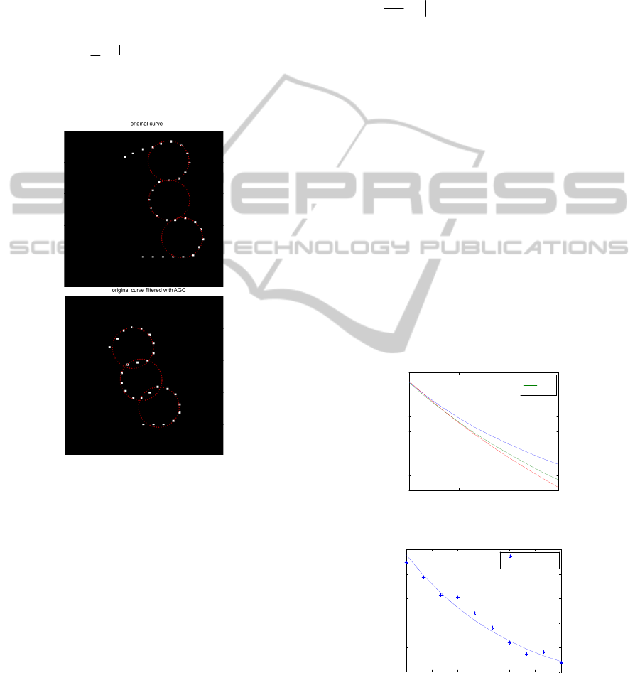
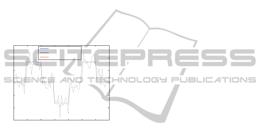
5.1 AGC of Curvature Processing
In this section two curves are presented. The first
one is a curve with constant curvature – part of a
circle (Fig. 16). The second is a combination of
straight lines and parts of circles with an opposite
curvature (Fig. 17).
The AGC parameters for both curves are:
() ; 20; 0.2
2
i
Wi k e k
γ
γ
γ
−
===,
(18)
with W having 5 elements.
Figure 17: AGC of fragmented curvature.
The first result represents spatial adaptation – the
curvature decreased (the radius of the curved
increased according to (16)), whereas the second
result represents curvature enhancement (or
emphasis). For presentation and comparison
purposes only, the result of the second curve is
multiplied by 1.87, to “compensate” for the
adaptation phenomenon – in order to correct
comparison between the original curve and the
filtered curve. Red circles have been added to Fig.
17 to emphasis the changes between the original
curve, and the result. According to (16), points that
are inside the circles have larger curvature than
points that are on the circle. T herefore, the edge
points (where a change in the curvature occurs) are
emphasized in the same way as at Fig. 4.
5.2 AGC of Size Processing
The two experiments of Roberts et al. were
reconstructed using Matlab and simulating the
perceived target size by using the AGC algorithm
presented in section 2 using parameters of:
2
( ) ( ) : 5, 0.00007
121
Wi k i whenk
γγ
=− ==
,
(19)
meaning that the lateral effect of W is a triangular
function with width of 121 elements.
First, experiment 1 was reconstructed. Target
was surrounded by 8 inducers at different radii
(varying from 5 to 20 pixels). This was checked for
near (30 pixels away from target), medium (40
pixels away from target) and far (50 pixels away
from target) inducers. Target radius was 10 pixels.
Target size (in pixels) as a function of inducer radius
and distance is shown at Fig. 18.
Second, experiment 3 was reconstructed. Target
was surrounded by variant number of inducers in
order to occupy an approximately constant
proportion (about 0.75) of the surround
circumference. Inducers were kept at a constant
radius and their distance from the target was
changed from 30 to 60 pixels. Target radius was 10
pixels. Target size (in pixels) as a function of
inducer distance is shown in Fig. 19. The solid line
in this figure is the best fit for the data.
5 10 15 20
-6
-5.5
-5
-4.5
-4
-3.5
-3
-2.5
-2
illusion magnitude as function of inducer radius
Inducer radus [pixels ]
illusion magnitude [pixels]
near
medium
far
Figure 18: Results of experiment 1 using AGC model.
30 35 40 45 50 55 60
-5.5
-5
-4.5
-4
-3.5
-3
g
Inducer dist anc e [pixels ]
illusion magnitude [pixels]
experiment results
-6+11.85e
(-x/21.28)
Figure 19: Results of experiment 3 using visual AGC
model.
AUTOMATIC GAIN CONTROL NETWORKS FOR MULTIDIMENTIONAL VISUAL ADAPTATION
171
0
10
20
30
40
50
0
10
20
30
40
50
0
2
4
6
8
10
x
Depth information
y
0 5 10 15 20 25 30 35 40 45 50
0
2
4
6
8
10
Depth information
x
0
10
20
30
40
50
0
20
40
60
10
15
20
25
x
Depth information after AGC filter
y
0 5 10 15 20 25 30 35 40 45
12
14
16
18
20
22
24
26
Depth information after AGC filter
x
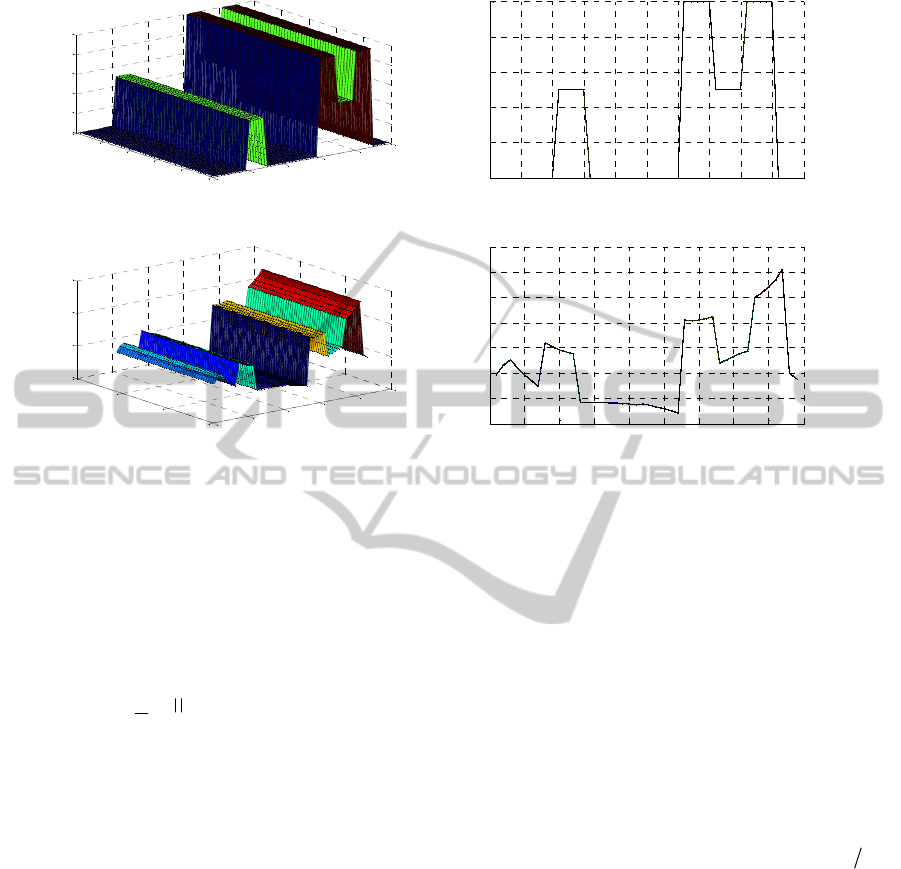
Figure 20: AGC processing of depth information. Input and output visual signals are displayed in the top and bottom rows,
respectively.
5.3 AGC of Depth Processing
We reconstruct Graham and Rogers’s experiment
using the visual AGC NN, implemented along the
visual dimension of depth, with:
() ; 1; 0.2
2
i
Wi k e k
γ
γ
γ
−
===,
(20)
where W has 11 elements.
For each point of the 3D original image the
depth is calculated relative to a point in the middle
of the image and with height of 50 pixels. Fig. 20
shows the results in both 3D and cross sections
view. As a result of the AGC, the left bar, which is
at the same depth as the right bar, is now perceived
closer.
6 DISCUSSION
Qualitatively speaking, important and interesting
events along curves, for example, consist only of
abrupt changes of orientation and curvature, as is
the case with other image attributes (dimensions).
Local maxima of curvature, and inflection points
(i.e. zero crossings of curvature) identify in this case
such events (see (Hoffman & Richards 1984),
(Koenderink & Doom 1982), (Richards et al. 1986)
and (Fischler & Bolles 1986)).
Therefore, it is reasonable to assume that visual
systems emphasize these changes and adapt to the
locally-constant value. This is indeed an important
feature of processing curvature (or other image
attributes) by adaptive NN endowed with the
characteristic of AGC. Curvature emphasis (as is
demonstrated in Fig. 17) and adaptation (as is
demonstrated in Fig. 16) occur simultaneously and
their extent can be controlled by varying the
parameter k of the NN hardwired connectivity.
Further, the effective range of interaction,
characterized in the hardwired network by
1
γ
,
becomes, due to the AGC of the nonlinear NN a
function of the slow rate of change (‘local DC’, i.e.
s
C of Eq. 6) along the image dimension processed
by the AGC NN, i.e. in the examples of Fig. 16 and
Fig. 17 the curvature.
Inspecting the results of size processing indicates
a good correspondence between the adaptive NN
response (Fig. 18 and Fig. 19) and the
psychophysical experimental results (Fig. 13 and
Fig. 14), both for the distance parameter and for the
size parameter. Such results should be expected due
to the dependency of AGC NN on these two
parameters as well, i.e. cells proximity and
specificity (in this case, objects’ size).
It is clear why increasing the inducer size
ICFC 2010 - International Conference on Fuzzy Computation
172

decreases the target perceived size. This is discussed
in section 2, and represents the size contrast effect of
the model. It is less obvious why farther positioned
inducers have stronger effect on target perceived
size, than that of the closer inducers (i.e. decreasing
the target size more effectively). The latter is due to
the mutual relation between the inducers. According
to the model of AGC visual processing, the cells
have a limited influence on their neighbors. If the
distance between cells is greater compared with W’s
effective width, then those cells will have a
minimum effect on each other (if any). When an
inducer is at a given distance
x
from the target, its
distance from the other inducers varies from 0 to
2
x
.
Thus, when distance increases, more and more
inducers are beyond the ‘influence zone’ of the other
inducers. This causes the perceived size of each
inducer to increase when the distance is increased.
Fig. 21 shows this phenomenon on the data of
experiment 1. Since the target is still inside the
‘influence zone’ of the inducers, and the size of the
inducers is now larger, the target seems smaller (the
size-contrast effect is enhanced).
When we add inducers while increasing the
distance (as in experiment 3), the target size is
reduced since each one of the inducers contribute to
the size-contrast effect.
Note that here we modelled only the target and
the inducers as objects with size. But, it is also
possible that the visual system treats the space
between the target and the inducers as an object with
size. In this case, if the space between the target and
the inducer is large, the inducer size has only a
secondary effect, and the target size is determined
mainly by the nearest object (for example see Fig.
22 - Delboeuf illusion. In this illusion, the target gets
smaller when the inducer diameter increases). This
model can explain also the moon size illusion.
30 32 34 36 38 40 42 44 46 48 50
3.9
3.95
4
4.05
4.1
4.15
4.2
4.25
inducers perceived size as a function of the distance from the target
Inducer distance [pixels]
inducers perceived size [pixels]
Figure 21: Results indicating that inducers perceived size
is increased at greater distances.
Figure 22: Delboeuf illusion.
7 CONCLUSIONS
Understanding the HVS and modelling certain
characteristics of it by adaptive NN is of a
considerable interest because of its potential use in
the design of intelligent computer vision and image
processing NN and systems. Because of the
complexity of the processes involved, and in order to
account for the vast volume of available
experimental data, there is need for relatively simple
models. As shown, the recurrent nonlinear adaptive
NN that exhibits AGC is relatively simple (only few
parameters) and versatile. It does not call for
postulating any components of neural circuitry more
complex than those well known to exist in biological
neural networks. It is important to stress that these
networks are sparsely connected. This fact allows
also to implement them sequentially by using Peano
– Hilbert scan for a quick and efficient processing
‘on the fly’ (for a review see (Jagadish 1990)). The
sparse NN proposed by us is in contrast to Hopfield-
type networks that are fully connected. The sparsely
(locally) connected NN can be also analyzed
theoretically (Shefer 1979).
Using the AGC model for all of the image base
dimensions (or other modalities for this matter)
provides great advantages. It constitutes a universal
and parsimonious model that explains how our
visual system processes visual information along its
various dimensions, before the later stage of
sequential “visual routines” is implemented. Having
this model allows us to process an image not only in
the intensity/spatio-temporal domain, but also along
all other dimensions as well. For example, given a
noisy curve, we can reduce the noise along the
curvature dimension with standard filters, such as
non-linear diffusion filter (Fig. 23).
The proposed visual AGC mechanism can
enhance existing schemes of intelligent image
processing with reference to enhancement of various
image attributes and features, i.e. curvature, size and
AUTOMATIC GAIN CONTROL NETWORKS FOR MULTIDIMENTIONAL VISUAL ADAPTATION
173
other image attributes. The decomposition of the
image into separable components is by no means the
only possible model of representation and
processing of images, and definitely not always the
optimal one. An alternative approach, introduced in
the context of image processing and computer vision
(Kimmel et al. 2000), (Sochen & Zeevi 1998),
considers an image to be a manifold embedded in
higher dimensional combined position (spatial)-
feature space. The features are the image attributes
or dimensions, such as color, curvature and size
mentioned above. Adaptation by means of nonlinear
gain control is executed in this case in the
multidimensional space in a unified manner. Such
manifolds of adaptive NN are yet to be further
investigated.
0 10 20 30 40 50 60 7
0
-0.03
-0.02
-0.01
0
0.01
0.02
0.03
original curve
noisy curve
curve after diffusion filter
Figure 23: Filtering a noisy curve with non-linear
diffusion filter (15 iterations) along the curvature
dimension.
REFERENCES
Abbott, L. F. et al., 1997. Synaptic Depression and
Cortical Gain Control. Science, 275(5297), 221-224.
Blakemore, C. & Campbell, F. W., 1969. On the existence
of neurones in the human visual system selectively
sensitive to the orientation and size of retinal images.
The Journal of Physiology, 203(1), 237-260.1.
Bradshaw, M. F., Parton, A. D. & Glennerster, A., 2000.
The task-dependent use of binocular disparity and
motion parallax information. Vision Research, 40(27),
3725-3734.
Bradshaw, M. F. & Rogers, B. J., 1996. The Interaction of
Binocular Disparity and Motion Parallax in the
Computation of Depth. Vision Research, 36(21),
3457-3468.
Bruckstein, A. M. & Zeevi, Y.Y., 1979. Analysis of
"integrate-to-threshold" neural coding schemes.
Biological Cybernetics, 34(2), 63-79.
Bruno, N. & Cutting, J. E., 1988. Minimodularity and the
perception of layout. Journal of Experimental
Psychology. General, 117(2), 161-170.
Carey, D. P., Harvey, M. & Milner, A. D., 1996.
Visuomotor sensitivity for shape and orientation in a
patient with visual form agnosia. Neuropsychologia,
34(5), 329-337.
Cavanagh, P., Arguin, M. & Treisman, A., 1990. Effect of
surface medium on visual search for orientation and
size features. Journal of Experimental Psychology:
Human Perception and Performance, 16(3), 479-491.
Coltheart, M., 1971. Visual feature-analyzers and
aftereffects of tilt and curvature. Psychological
Review, 78(2), 114-121.
Dijkstra, T. M. H. et al., 1995. Perception of three-
dimensional shape from ego- and object-motion:
Comparison between small- and large-field stimuli.
Vision Research, 35(4), 453-462.
Ding, J. & Sperling, G., 2006. A gain-control theory of
binocular combination. Proceedings of the National
Academy of Sciences of the United States of America,
103(4), 1141-1146.
Dobbins, A., Zucker, S.W. & Cynader, M. S., 1987.
Endstopped neurons in the visual cortex as a substrate
for calculating curvature. Nature, 329, 438-441.
Du Croz, J. J. & Rushton, W. A. H., 1966. The separation
of cone mechanisms in dark adaptation. The Journal of
Physiology, 183(2), 481-496.
Enns, J. T. & Rensink, R. A., 1990a. Influence of scene-
based properties on visual search. Science (New York,
N.Y.), 247(4943), 721-723.
Enns, J. T. & Rensink, R. A., 1990b. Sensitivity to Three-
Dimensional Orientation in Visual Search.
Psychological Science, 1(5), 323-326.
Fischler, M. A. & Bolles, R. C., 1986. Perceptual
organization and curve partitioning. IEEE Trans.
Pattern Anal. Mach. Intell., 8(1), 100-105.
Gibson, J.J., 1937. Adaptation with negative after-effect.
Psychological Review, 44(3), 222-244.
Ginosar, R., Hilsenrath, O. & Zeevi, Y. Y., 1992. United
States Patent: 5144442 - Wide dynamic range camera.
Graham, M. & Rogers, B. J., 1982. Simultaneous and
successive contrast effects in the perception of depth
from motion-parallax and stereoscopic information.
Perception, 11(3), 247 – 262.
Hancock, S. & Peirce, J. W., 2008. Selective mechanisms
for simple contours revealed by compound adaptation.
Journal of Vision, 8(7), 1-10.
Hochstein, S. & Ahissar, M., 2002. View from the top:
hierarchies and reverse hierarchies in the visual
system. Neuron, 36(5), 791-804.
Hoffman, D. D. & Richards, W.A., 1984. Parts of
recognition. Cognition, 18(1-3), 65-96.
Hubel, D. H. & Wiesel, T. N., 1979. Brain mechanisms of
vision. Scientific American, 241(3), 150-162.
Hubel, D. H. & Wiesel, T. N., 1968. Receptive fields and
functional architecture of monkey striate cortex. The
Journal of Physiology, 195(1), 215-243.
Hubel, D. H. & Wiesel, T. N., 1962. Receptive fields,
binocular interaction and functional architecture in the
cat's visual cortex. Journal of Physiology (London),
160(1), 106-154.
ICFC 2010 - International Conference on Fuzzy Computation
174

Hubel, D. H. & Wiesel, T. N., 1970. Stereoscopic Vision
in Macaque Monkey: Cells sensitive to Binocular
Depth in Area 18 of the Macaque Monkey Cortex.
Nature, 225, 41-42.
Inui, T. et al., 2000. Neural substrates for depth perception
of the Necker cube; a functional magnetic resonance
imaging study in human subjects. Neuroscience
Letters, 282(3), 145-148.
Jagadish, H. V., 1990. Linear clustering of objects with
multiple attributes. In Proceedings of the 1990 ACM
SIGMOD international conference on Management of
data, 332-342.
Kimmel, R., Malladi, R. & Sochen, N., 2000. Images as
Embedded Maps and Minimal Surfaces: Movies,
Color, Texture, and Volumetric Medical Images.
International Journal of Computer Vision, 39(2), 111-
129.
Koenderink, J. J. & Doom, A. J .V., 1982. The shape of
smooth objects and the way contours end. Perception,
11(2), 129 – 137.
Koenderink, J. J. & Doorn, A. J. V., 1987. Representation
of local geometry in the visual system. Biological
Cybernetics, 55(6), 367-375.
Krauskopf, J. & Mollon, J. D., 1971. The independence of
the temporal integration properties of individual
chromatic mechanisms in the human eye. The Journal
of Physiology, 219(3), 611-623.
Lu, Z. & Sperling, G., 1996. Contrast gain control in first-
and second-order motion perception. Journal of the
Optical Society of America A, 13(12), 2305-2318.
Parent, P. & Zucker, S.W., 1989. Trace Inference,
Curvature Consistency, and Curve Detection. IEEE
Transactions on Pattern Analysis and Machine
Intelligence, 11(8), 823-839.
Ratliff, F., 1965. Mach bands: Quantitative studies on
neural networks in the retina. Holden-Day inc.
Richards, W., Dawson, B. & Whittington, D., 1986.
Encoding contour shape by curvature extrema. Journal
of the Optical Society of America A, 3(9), 1483-1491.
Riggs, L. A., 1973. Curvature as a Feature of Pattern
Vision. Science, 181(4104), 1070-1072.
Roberts, B., Harris, M.G. & Yates, T.A., 2005. The roles
of inducer size and distance in the Ebbinghaus illusion
(Titchener circles). Perception, 34(7), 847 – 856.
Rogers, B. J. & Graham, M., 1979. Motion parallax as an
independent cue for depth perception. Perception,
8(2), 125 – 134.
Schwartz, O. & Simoncelli, E. P., 2001. Natural signal
statistics and sensory gain control. Nat Neurosci, 4(8),
819-825.
Shefer, M., 1979. AGC models for retinal signal
processing. M.Sc. Thesis. Technion.
Sochen, N. & Zeevi, Y. Y., 1998. images as manifolds
embedded in a spatial feature non euclidean space.
IEEE ICIP, 166-170.
Stromeyer, C. F. & Riggs, L.A., 1974. Curvature
Detectors in Human Vision? Science, 184(4142),
1199-1201.
Sutherland, N. S., 1968. Outlines of a Theory of Visual
Pattern Recognition in Animals and Man. Proceedings
of the Royal Society of London. Series B, Biological
Sciences, 171(1024), 297-317.
Treisman, A. M. & Gormican, S., 1988. Feature analysis
in early vision: Evidence from search asymmetries.
Psychological Review, 95(1), 15-48.
Wainwright, M. J., 1999. Visual adaptation as optimal
information transmission. Vision Research, 39(23),
3960-3974.
Weltsch-Cohen, Y., 2002. AGC models for signal
processing in the primary visual cortex. M.Sc. Thesis.
Technion.
Wolfe, J. M. et al., 2003. Changing your mind: On the
contributions of top-down and bottom-up guidance in
visual search for feature singletons. Journal of
Experimental Psychology: Human Perception and
Performance, 29(2), 483-502.
Zeevi, Y. Y., Ginosar, R. & Hilsenrath, O., 1995. United
States Patent: 5420637 - Dynamic image
representation system.
Zeevi, Y. Y. & Kronauer, E. R., 1985. Reorganization and
diversification of signals in vision. EEE transactions
on systems, man, and cybernetics, 15(1), 91-101.
Zeevi, Y. Y. & Mangoubi, S.S., 1978. Noise suppression
in photoreceptors and its relevance to incremental
intensity thresholds. Journal of the Optical Society of
America, 68 (12), 1772-1776.
Zucker, S. W. et al., 1988. The Organization Of Curve
Detection: Coarse Tangent Fields And Fine Spline
Coverings. In Computer Vision., Second International
Conference, 568-577.
AUTOMATIC GAIN CONTROL NETWORKS FOR MULTIDIMENTIONAL VISUAL ADAPTATION
175
