HOW CAN NEURAL NETWORKS SPEED UP ECOLOGICAL

REGIONALIZATION FRIENDLY?

Replacement of Field Studies by Satellite Data using RBFs

Manolo Cruz, Mois

es Esp

ınola

Applied Computing Group, University of Almer

ıa, 04120 Almer

ıa, Spain

Rosa Ayala, Mercedes Peralta, Jos

e Antonio Torres

Computers and Environment Research Group, University of Almer

ıa, 04120 Almer

ıa, Spain

Keywords:

Neural network, RBF, Remote sensing, Ecological regionalization.

Abstract:

The aim of this work is to present an application of the Radial Basis Functions Nets (RBFs) for simplifying

and reducing the cost of ecological regionalization. The process speeds up and replaces the classic means

of obtaining ecological variables through ﬁeld studies. The radial basis function networks were applied to

estimate ﬁeld data remotely, using data captured by the Landsat satellite and correlating it with ecological

variables in order to substitute for them in the regionalization process. This approach substantially reduces

the time and cost of ecological regionalization, limiting ﬁeld studies and automating the generation of the

ecological variables. The technique could be applied without restriction to map vegetation in any other area

for which satellite coverage exists.

1 INTRODUCTION

The need or sound environmental management of a

particular territory requires a sufﬁcient and integrated

understanding of the resources there, and the interre-

lationships with the natural and human elements that

act upon it (Moreira, 2000). Nevertheless, and in spite

of the enormous effort to generate this thematic in-

formation, the reality is that the results are still unsa-

tisfactory in terms of environmental planning (Pablo,

2000).

This situation has led the majority of the spa-

nish regions to prepare their own environmental carto-

graphic information. Ecological regionalization was

developed with the aim of providing useful informa-

tion about the web of relationships between various

natural elements in an area over both space and time.

This type of mapping attempts to integrate the most

relevant environmental aspects of a territory in or-

der to identify patterns that allow the structure and

operation of a territory to be understood, classify-

ing them into a series of units called environmen-

tals. These units are characterized by the close ho-

mogeneity of the environmental variables considered

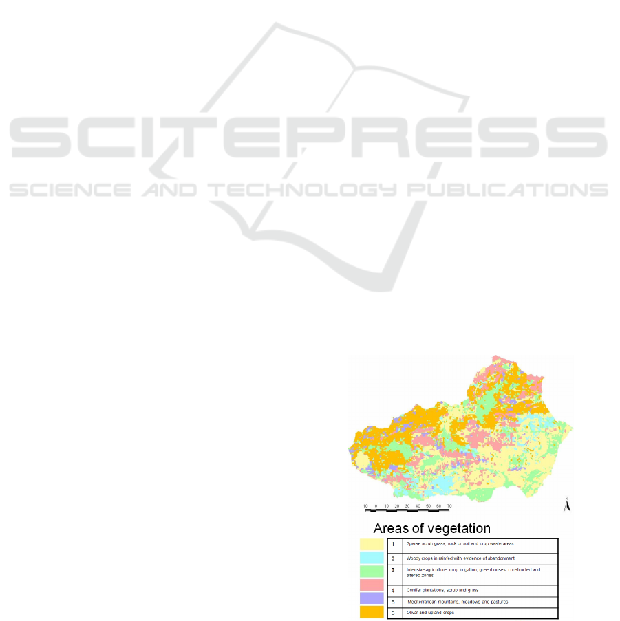
(Naiman et al., 1992). Figure 1 shows the vegetation

map based on the ecological variables used for this

study.

Figure 1: Vegetation map based on the ecological variables

used in this study area (Almer

ıa and Granada, Spain).

Ecological regionalizations (also referred to as

ecoregions, biogeographic regions land classes and

295

Cruz M., Espínola M., Ayala R., Peralta M. and Torres J..

HOW CAN NEURAL NETWORKS SPEED UP ECOLOGICAL REGIONALIZATION FRIENDLY? - Replacement of Field Studies by Satellite Data using

RBFs.

DOI: 10.5220/0003062402950300

In Proceedings of the International Conference on Fuzzy Computation and 2nd International Conference on Neural Computation (ICNC-2010), pages

295-300

ISBN: 978-989-8425-32-4

 2010 SCITEPRESS (Science and Technology Publications, Lda.)

environmental classiﬁcations, environmental do-

mains, ecological land units,) play important roles in

process of resource management by grouping loca-

tions with similar environmental variables (Snelder

et al., 2010). Undertaking this kind of ecological

regionalization requires the following environmental

data (Loveland and Merchant, 2004):

• Climatic: obtained from the state meteorological

agencies, and comprising time series running over

several years.

• Geological: obtained from ﬁeld studies to mea-

sure rainfall and soil composition.

• Vegetation cover: obtained from ﬁeld studies of

vegetation cover in order to tabulate the presence

of different species and vegetation types.

• Land Use: obtained from ﬁeld studies of land use

in the study area.

This information is used by the various technical

environmental departments for ecological regionali-

zation, using statistical techniques. Nonetheless, un-

til now, it has still been necessary to undertake va-

rious ﬁeld studies to keep the environmental infor-

mation up-to-date, and this makes it quite difﬁcult to

have an up-to-date ecological map in a short period

of time. Thus, with the dual aims of unifying the in-

formation sources used to draw ecological maps, and

simplifying and reducing the cost of obtaining many

of these data, the present study (undertaken within the

framework of the SOLERES project ﬁnanced by the

Spanish Ministry of Science and Technology) applies

models of neural networks that use cheaper and up-to-

date satellite data to construct ecological maps, whilst

maintaining the procedures for constructing this car-

tography. The study is not designed to substitute one

set of ecological variables for another, but to ﬁnd an

alternative procedure to construct the variables.

2 NEURAL NETS AND REMOTE

SENSING

Neural networks have proved their potential as tools

for classiﬁcation and approximation of functions for

over ten years. The advantages over other analytical

and statistical techniques stems from their capacity to

handle large volumes of high-dimensional data, the

capacity to work with scarce, changing and/or contra-

dictory data, and their independence from the statis-

tical characteristics of the sample. Moreover, neural

networks exhibit a signiﬁcant capacity for generalisa-

tion that means they become powerful tools for stu-

dying the dynamics of atmosphere and climate from

Figure 2: Basic structure of an RBF.

satellite images, for classifying vegetation types and

other related activities (Richards, 1993).

Radial basis function networks (RBFs) (Poggio

and Girosi, 1990) were developed later than MLPs

and, from an operational point of view, have certain

advantages over MLPs, such as faster training and an

internal structure that allows better understanding of

the relationships between variables, and therefore, a

better understanding of how the network functions.

Figure 2 shows the three basic levels of an RBF:

• An input layer, in which the characteristics vector

is applied to each and every element of the follo-

wing level.

• A radial basis function net level, called the hidden

layer unit, which computes the expression:

RBF

(~x) = e

−

~x−~c

where c

is the centroid of the radial base func-

tion and σ is the scope parameter (measuring the

spread) of each radial base function.

• An integration or output layer, where the results of

each RBF is adjusted/weighted, to give the output

of the net, according to the function:

Y =

∑

RBF

(~x) − b

where w

is the weighting parameter and b is the

threshold value.

The training phase of an RBF consists of selec-

ting the centroids c

and the values of the weights

that minimise the error produced by the network

for the training data set. RBFs exhibit certain ad-

vantages over other types of net like MLPs, such as

the speed of training. Nevertheless, they have certain

drawbacks, such as the fact that, to solve a particular

problem, RBFs require a greater number of neurons

and so a larger computing effort. The application of

RBFs for the present study is justiﬁed by the fact that

ICFC 2010 - International Conference on Fuzzy Computation

296

many training phases are required and this would take

a long time using other methods.

3 DESCRIPTION OF THE WORK

The study area comprised the provinces of Almer

ıa

and Granada, in south-eastern Spain (southern Eu-

rope). The study was designed in several phases:

1. Determine the ecological variables that are suita-

ble for approximation using satellite data.

2. Obtain satellite data to correspond with each value

of the ecological variable.

3. Train and run simulations of the neural networks.

4. Compare the results obtained with the expected

values.

3.1 Determine the Ecological Variables

that are Suitable for Approximation

using Satellite Data

The data for these variables were obtained from ﬁeld

studies undertaken by technical staff working for the

Administration. The data are updated periodically

using ﬁeld data or aerial photographs. The informa-

tion for each variable is obtained by weighting the sur-

face area of vegetation cover for each vegetation type

within each 1x1Km sector. This produces numerical

values for each 1x1Km sector and for each variable,

which represents the percentage cover of each vege-

tation type included in this study, expressed over the

interval [0,100].

The area of study includes a great diversity of

woodland landscapes, ranging from wet woodlands to

desert landscapes containing a wide range of ecosys-

tems, dominated by high mountain ranges, subtropi-

cal maritime area and subdesert plains. In this way,

the study enabled an analysis of landscapes contai-

ning a wide variety of vegetation types (Snelder et al.,

2007). Table 1 shows the ecological variables used.

3.2 Obtain Satellite Data to Correspond

with Values of Ecological Variables

Improvements in remote sensing technologies and

the use of geographic information system (GIS), are

increasingly allowing us to develop indicators that

can be used to monitor and assess ecosystem condi-

tion and change at multiple scales (Revenga, 2005).

The Landsat satellite includes a TM sensor (Thematic

Mapper) that captures data over seven bands of the

electromagnetic spectrum. The sensor is linked to te-

rritorial studies whose principal focus is environmen-

tal. Its orbit, synchronous with the sun, is atan altitude

of 705km and has a period of 98.9 minutes, totalling

14 ﬂights daily around the earth.

Table 1: List of ecological variables used in the study.

N Concept

01 Built-up and disturbed areas

02 Wetlands and open water

03 River corridors vegetation

04 Herbaceous crops without irrigation

05 Olive plantations

06 Other woody crops without irrigation

07 Forced crops under plastic

08 Other herbaceous crops under irrigation

09 Woody crops under irrigation

10 Herbaceous and woody crops

11 Mosaic of woody crops (no irrigation)

12 Herbaceous and woody crops (irrigation)

13 Mosaic of woody crops under irrigation

14 Mosaic of crops under irrigation or not

15 Herbaceous crops and pastures

16 Herbaceous crops and woody vegetation

17 Woody crops and pastures

18 Woody crops and woody vegetation

19 Mosaics of crops and natural vegetation

20 Abandoned woody crops

21 Mediterranean oak woodland

22 Conifers

23 Other tree species and mixtures

24 Dense matorral + dense oak wood

25 Dense matorral + scattered oaks

26 Dense matorral + dense conifers

27 Dense matorral + scattered conifers

28 Dense matorral + mixed tree species

29 Scattered matorral + dense oak wood

30 Scattered matorral and oaks

31 Scattered matorral + dense conifers

32 Scattered matorral + scattered conifers

33 Scattered matorral + mixed tree species

34 Pasture + dense Mediterranean oakwood

35 Pasture + scattered Mediterranean oaks

36 Pasture + dense conifers

37 Pasture + scattered conifers

38 Pasture + other tree species or mixed

39 Zones subject to ﬁerce erosion or ﬁres

40 Dense matorral

41 Scattered matorral with pasture

42 Scattered matorral (pasture and rock)

43 Continuous pasture

44 Pasture with rock or soil clearings

45 Beaches, dunes and sandbanks

HOW CAN NEURAL NETWORKS SPEED UP ECOLOGICAL REGIONALIZATION FRIENDLY? - Replacement of

Field Studies by Satellite Data using RBFs

297

In order to capture all of the study area, we needed

three Landsat scenes. These satellite images were

used to make a mosaic, and the image was trimmed

with a vector of the outline of Almer

ıa and Granada

provinces, giving the processed image that served as

the basis for our study (vegetation data and remote

sensing matching).

To do this, the original image was trimmed using a

window of 33x33 pixels (990m2). The displacement

error (the 10m2 missing from the 1000m2) was co-

rrected by alternating the 33x33 pixel window with

another measuring 34x34 pixels, every two passes.

The result was an image of 241x157 pixels, with a

spatial resolution of 1000x1000m.

Following the same procedure, the median, mean

and 30 percentile of each window of the original

image was also calculated. This was stored, for each

of its seven layers, in a matrix. By this means, we

generated 21 variables with which to calculate each

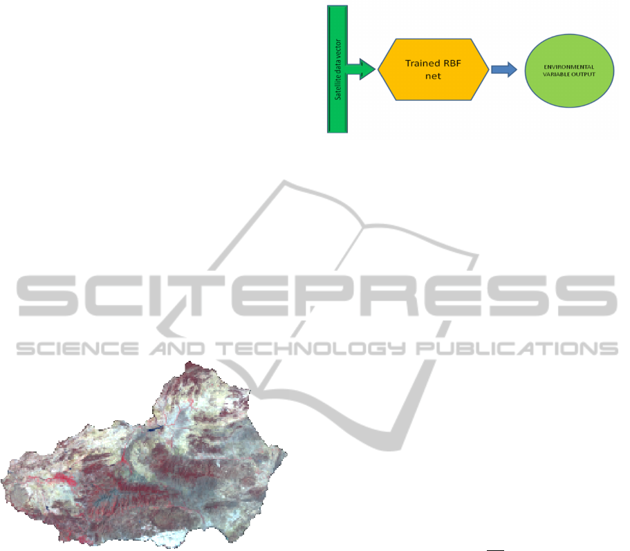
of the ecological variables of vegetation cover. Figure

3 shows Almer

ıa and Granada provinces in LandSat

data.

Figure 3: Detail of the study area using LandSat data.

3.3 Train and Run Simulations of the

Neural Networks

The next step was to train a series of RBF neural net-

works to relate each ecological variable to the pro-

cessed satellite data. For each ecological variable,

there are 21,905 ground surface samples available,

each representing 1x1 Km, for which statistical in-

formation from the seven satellite bands has been ge-

nerated. In this way, each sector yields 21 characte-

ristics describing it. So, for each variable we have a

data model of 21,905x21, with 21,905 desired results,

which are the data from which we will train the neural

net.

Modelling of each of the 45 ecological variables

involved repeating the construction of an RBF net 32

times, using 70% of the data as the training data set

Figure 4: Detail of the process undertaken by the neural net.

and the remaining 30% as the calibration data set. The

division of data into these two datasets was done at

random in every case. In total, 1440 networks were

trained.

Once trained, the input to the neural net is changed

to the satellite data, and its output offers an approxi-

mate value of the environmental variable for which it

has been trained. This technique increases the possi-

bility of ﬁnding a net that satisfactorily approximates

to the ecological variable. The radial basis function

network uses a random parameter over the interval [0,

1.5]. Figure 4 shows the process undertaken by the

neural net.

3.4 Compare the Results obtained with

the Expected Values

Once the networks are constructed, the results ob-

tained for the calibration data set are compared with

the expected values and two measures are calculated:

1. The precision, obtained using the formula:

pr =

where e is the number of times that the output of

the neural net coincides with the expected output,

with an error of ±0.005, and C is the calibration

data set. The training data set is not taken into

consideration because the precision obtained with

the training set would be close to 1 and this would

distort the precision of the calibration data set.

2. The variance between the expected results and

those obtained indicates the ecological variables

for which conﬁdence in the approximation is

sufﬁciently high. To calculate variance, both ex-

pected and obtained results are normalised to a

range [0,1] and the variance of the difference in

the absolute values is calculated.

The process was programmed in Matlab, using a

desktop computer with 4 core architecture and 8 GB

of memory. The program took 48 hours of inten-

sive calculations. An improvement in the calculation

ICFC 2010 - International Conference on Fuzzy Computation

298

time would be achieved using other computer archi-

tectures.

4 RESULTS

The most obvious ﬁnding of the experiment is that

the result was positive for all the ecological variables,

except variable 34 (pasture and dense Mediterranean

oak woodland) and variable 37 (pasture with scattered

conifers). The neural networks obtained ﬁt the be-

haviour of the ecological variables with a precision of

0.8 and variance of less than 0.03 in every case. For

the remaining two ecological variables that could not

be simulated, had given training networks with a peak

precision of 0.70 for the ﬁrst and 0.42 in the second.

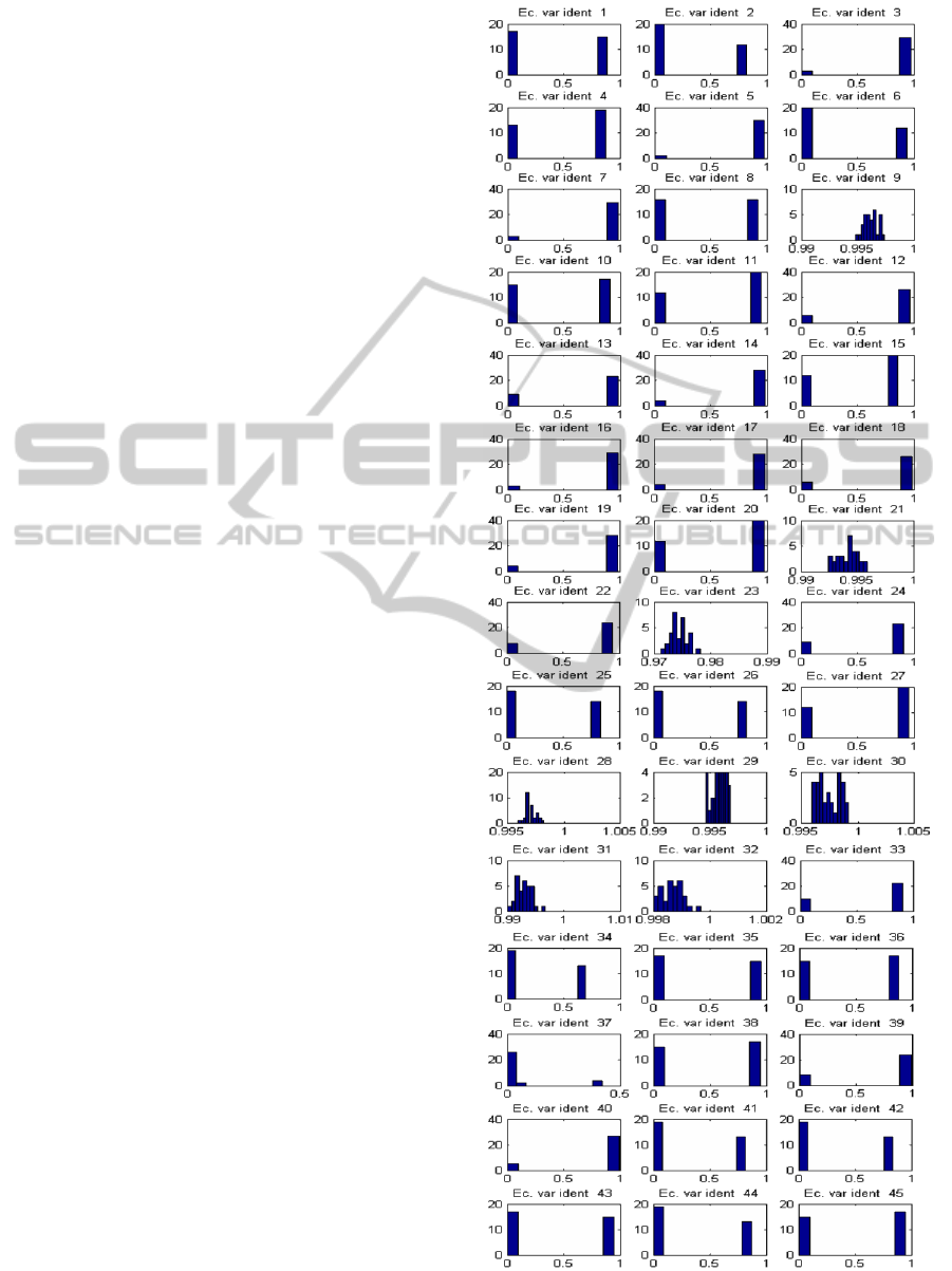
Figure 5 shows the distribution of the experiment pre-

cision by variable.

A priori, the result is not explained by the na-

ture of the variable and we ﬁnd the explanation in

the procedure used to choose the training and cali-

bration sets: the choice is made at random and with a

relatively small frequency of non-null data, the distri-

bution between the training and calibration data sets

is signiﬁcant for the precision of the net. Thus, for

example, if we use all the non-null data in the training

phase, we will obtain a precision of 0.9998 and a va-

riance of 0.0001 for variable 34; and a precision of

0.9983 and variance of 0.0016 for variable 37. Ta-

ble 2 shows the relative frequency of non-null data by

variable.

Excluding variables 34 and 37, the number of ex-

periments that generated networks of an acceptable

precision was, on average, 68%. 70% of the varia-

bles developed at least 53% precise neural networks.

This ﬁnding permits discussion of whether the model

of ﬁtting ecological variable using Landsat data and

RBF networks is sound. A signiﬁcant number of ex-

periments were undertaken for each variable, varying

the training data set and this achieved good results,

in the majority of cases, improving as the quantity of

non-null data increases for the ecological variable in

question.

With respect to the parameters of the network,

within the interval [0,1.5] the parameter scope does

not appear to be a determining factor in achieving a

better result. It is relevant to point out that, in a sig-

niﬁcant proportion of cases, the neural networks did

not manage to approximate to the associated ecologi-

cal variable. This situation is due to the nature of the

data for each variable and the randomness of selecting

data during each training process.

From an environmental point of view, organiza-

tion of the data into ecological variables and its subse-

Figure 5: Distribution of the experiment precision by

variable.

HOW CAN NEURAL NETWORKS SPEED UP ECOLOGICAL REGIONALIZATION FRIENDLY? - Replacement of

Field Studies by Satellite Data using RBFs

299

Table 2: Relative frequency of non-null data.

id 01 id 02 id 03 id 04 id 05

0,115 0,036 0,024 0,308 0,179

id 06 id 07 id 08 id 09 id 10

0,164 0,052 0,129 0,057 0,176

id 11 id 12 id 13 id 14 id 15

0,030 0,128 0,021 0,061 0,013

id 16 id 17 id 18 id 19 id 20

0,083 0,004 0,093 0,049 0,014

id 21 id 22 id 23 id 24 id 25

0,017 0,145 0,015 0,012 0,018

id 26 id 27 id 28 id 29 id 30

0,015 0,024 0,006 0,066 0,097

id 31 id 32 id 33 id 34 id 35

0,166 0,174 0,046 0,003 0,004

id 36 id 37 id 38 id 39 id 40

0,002 0,006 0,001 0,091 0,048

id 41 id 42 id 43 id 44 id 45

0,116 0,583 0,049 0,011 0,006

quent substitution using satellite data can be success-

fully achieved, as proved by the experience in the

classiﬁcation of vegetation types using the LandSat

data.

In addition, at least in the study zone, there is

no noticeable interaction between various vegetation

covers to complicate the training of the networks

which, in other situations, would have to be studied.

This situation may be due in part to the values ob-

tained: for each quadrat of land, the values indicate a

dominant vegetation type, so that 90% of the samples

have a vegetation cover of more than 41.9, while 50%

of cases have an vegetation cover exceeding 68.8. In

such a situation, the information obtained from the

satellite data is representing, in the majority of cases,

the dominant characteristic and for this reason, there

are no undesired interactions. In addition, the matrix

contains a large number of nil or very low data values:

92.3% of data are zero and only 55,800 data of a total

of 985,725 in the matrix, have values above 5.

5 CONCLUSIONS

As a ﬁnal point, the approximation functions of the

ecological variables developed here using radial basis

function networks could be used in subsequent years

to study changes in vegetation cover. Although the

vegetation cover changes seasonally, it is also true that

the experiment could be repeated for different seasons

of the year, so long as this cover existed.

The use of Landsat data in this case reduces ﬁeld

studies in at least 30%. Neural networks can recog-

nize geographical locations with similar vegetation

characteristics at any given time. This situation will

allow work teams to to study the Landsat information

previously available and improve the work on a sur-

face, saving costs.

From a technical point of view, the study also co-

rroborates the need for a precise study of the training

data set in order to achieve a precise training so

that the results are consistent with the environmen-

tal model simulated. The results conﬁrm our working

hypothesis that supports the viability of a computation

process of ecological variables that uses satellite data

that could substitute for the traditional ﬁeld studies.

ACKNOWLEDGEMENTS

This work has been supported by the EU (FEDER)

and the Spanish MICINN under grant of TIN2007-

61497 and TIN2010-1558 projects.

REFERENCES

Loveland, T. R. and Merchant, J. M. (2004). Ecoregions and

ecoregionalization: geographical and ecological pers-

pectives. In Environmental Management 34. Springer

New York.

Moreira, J. (2000). Reconocimiento biof

ısico de espa-

cios naturales protegidos. Parque natural Sierras

Subb

eticas. Junta de Andaluc

ıa, Sevilla, 1st edition.

Naiman, R., Loranrich, D., Beechie, T., and Ralph, S.

(1992). General principles of classiﬁcation and the

assessment of conservation potential in rivers. In

River Conservation and Management. John Wiley and

Sons.

Pablo, C. D. (2000). Cartograf

ıa ecol

ogica: conceptos y

procedimientos para la representaci

on espacial de eco-

sistemas. In Bolet

ın de la Real Sociedad Espaola de

Historia Natural. Real Sociedad Espaola de Historia

Natural.

Poggio, T. and Girosi, F. (1990). A theory of networks for

approximation and learning. In Proceedings of the

IEEE 78. Massachusetts Institute of Technology.

Revenga, C. (2005). Developing indicators of ecosystem

condition using geographic information systems and

remote sensing. In Regional Environmental Change

5. Springer Berlin and Heidelberg.

Richards, J. (1993). Remote sensing digital image analysis.

An introduction. Springer-Verlag, Berlin, 2nd edition.

Snelder, T., Leathwick, J., and Dey, K. (2007). A proce-

dure for making optimal selection of input variables

for multivariate environmental classiﬁcations. In Con-

servation Biology 21. National Institute of Water and

Atmospheric Research.

Snelder, T., Lehmann, A., Lamouroux, N., Leathwick, J.,

and Allenbach, K. (2010). Effect of classiﬁcation

procedure on the performance of numerically deﬁned

ecological regions. In Environmental Management 45.

Springer New York.

ICFC 2010 - International Conference on Fuzzy Computation

300