
ALGORITHMS FOR EVOLVING NO-LIMIT
TEXAS HOLD’EM POKER PLAYING AGENTS
Garrett Nicolai
Dalhousie University, Halifax, Canada
Robert Hilderman
Department of Computer Science, University of Regina, Regina, Canada
Keywords:
Poker, Evolutionary algorithms, Evolutionary neural networks.
Abstract:
Computers have difficulty learning how to play Texas Hold’em Poker. The game contains a high degree of
stochasticity, hidden information, and opponents that are deliberately trying to mis-represent their current state.
Poker has a much larger game space than classic parlour games such as Chess and Backgammon. Evolutionary
methods have been shown to find relatively good results in large state spaces, and neural networks have been
shown to be able to find solutions to non-linear search problems. In this paper, we present several algorithms
for teaching agents how to play No-Limit Texas Hold’em Poker using a hybrid method known as evolving
neural networks. Furthermore, we adapt heuristics such as halls of fame and co-evolution to be able to handle
populations of Poker agents, which can sometimes contain several hundred opponents, instead of a single
opponent. Our agents were evaluated against several benchmark agents. Experimental results show the overall
best performance was obtained by an agent evolved from a single population (i.e., with no co-evolution) using
a large hall of fame. These results demonstrate the effectiveness of our algorithms in creating competitive
No-Limit Texas Hold’em Poker agents.
1 INTRODUCTION
In the field of Artificial Intelligence, games have at-
tracted a significant amount of research. Games are
of interest to researchers due to their well defined
rules and success conditions. Furthermore, game-
playing agents can be easily benchmarked, as they can
play their respective games against previously-created
agents, and an objective skill level can be determined.
Successful agents have been developed for de-
terministic parlour games such as Chess (Camp-
bell et al., 2002; Donninger and Lorenz, 2005)
and Checkers(Samuel, 1959; Schaeffer et al., 1992),
and stochastic games such as Backgammon(Tesauro,
2002). These agents are capable of competing at the
level of the best human players.
These games all have one key aspect in common:
they all involve perfect information. That is, all play-
ers can see all information relevant to the game state
at all times. Recently, games of imperfect informa-
tion, such as Poker(Barone and While, 1999; Beattie
et al., 2007; Billings et al., 2002; Johanson, 2007) has
started to attract attention in the research community.
Unlike Chess and Checkers, there are certain, where
all information is available to all players, Poker in-
volves deception and hidden information. Part of the
allure of card games in general, and Poker in partic-
ular is that a player must take risks, based on incom-
plete information.
This hidden information creates a very large deci-
sion space, with many potential decision paths. The
most often studied variant of Poker is a variant known
as Limit Texas Hold’em (Barone and While, 1999;
Billings et al., 2002; Johanson, 2007). This variant
limits the size of the decision space by limiting the po-
tential decisions available to an agent. Another vari-
ant, known as No-Limit Texas Hold’em (Beattie et al.,
2007; Booker, 2004), changes only one rule, but re-
sults in many more potential decisions for an agent,
and consequently, a much larger decision space.
In this paper, we present an algorithm for creat-
ing an agent to play No-Limit Texas Hold’em. Rather
than reduce the decision space, we use evolution-
ary algorithms (Samuel, 1959; Schaeffer et al., 1992;
20
Nicolai G. and Hilderman R..
ALGORITHMS FOR EVOLVING NO-LIMIT TEXAS HOLD’EM POKER PLAYING AGENTS.
DOI: 10.5220/0003063000200032
In Proceedings of the International Conference on Evolutionary Computation (ICEC-2010), pages 20-32
ISBN: 978-989-8425-31-7
Copyright
c
2010 SCITEPRESS (Science and Technology Publications, Lda.)

Thrun, 1995; Pollack and Blair, 1998; Barone and
While, 1999; Kendall and Whitwell, 2001; Lubberts
and Miikkulainen, 2001; Tesauro, 2002; Hauptman
and Sipper, 2005; Beattie et al., 2007) to teach our
agents a guided path to a good solution. Evolutionary
algorithms mimic natural evolution, and reward good
decisions while punishing less desirable ones. Our
agents use neural networks to make decisions on how
to bet under certain circumstances, and through iter-
ative play, and minor changes to the weights of the
neural networks, our agents learn to play No-Limit
Texas Hold’em.
2 RULES OF NO LIMIT TEXAS
HOLD’EM
No-Limit Texas Hold’em is a community variant of
the game of Poker. Each player is dealt two cards, re-
ferred to as hole cards. After the hole cards are dealt,
a round of betting commences, whereby each player
can make one of three decisions: fold, where the
player chooses to stop playing for the current round;
call, where the player chooses to match the current
bet, and keep playing; and raise, where the player
chooses to increase the current bet. This is where
No-Limit Texas Hold’em differs from the Limit vari-
ant. In Limit Texas Hold’em, bets are structured,
and each round has a maximum bet. In No-Limit
Texas Hold’em, any player may bet any amount, up
to and including all of his remaining money, at any
time. After betting, three community cards, collec-
tively known as the flop are dealt. The community
cards can be combined with any player’s hole cards to
make the best 5-card poker hand. After the flop, an-
other betting round commences, followed by a fourth
community card, the turn. Another betting round en-
sues, followed by a final community card, known as
the river, followed by a final betting round. If, at any
time, only one player remains due to the others fold-
ing, this player is the winner, and a new round com-
mences. If there are at least two players remaining
after the final betting round, a showdown occurs: the
players compare their hands, and the player with the
best 5-card Poker hand is declared the winner.
3 RELATED WORK
Research into computer Poker has progressed slowly
in comparison with other games, so Poker does not
have as large an established literature.
3.1 Limit Texas Hold’em Poker
The Computer Poker Research Group at the Univer-
sity of Alberta is the largest contributor to Poker re-
search in AI. The group recently created one of the
best Poker-playing agents in the world, winning the
2007 Poker Bot World Series (Johanson, 2007).
Beginning with Loki (Billings et al., 1999), and
progressing through Poki (Billings et al., 2002) and
PsOpti (Billings et al., 2003), the University of
Alberta has concentrated on creating Limit Texas
Hold’em Poker players. Originally based on oppo-
nent hand prediction through limited simulation, each
generation of Poker agents from the UACPRG has
modified the implementation and improved upon the
playing style of the predecessors. The current agents
(Johanson, 2007; Schauenberg, 2006) are mostly
game theoretic players that try to minimize loss while
playing, and have concentrated on better observa-
tion of opponents and the implementation of counter-
strategies. The current best agents are capable of de-
feating weak to intermediate human players, and can
occasionally defeat world-class human players.
3.2 No-limit Texas Hold’em Poker
No-Limit Texas Hold’em Poker was first studied in
(Booker, 2004), where a rule-based system was used
to model players. The earliest agents were capable of
playing a very simple version of two-player No-Limit
Texas Hold’em Poker, and were able to defeat several
benchmark agents. After modifying the rules used to
make betting decisions, the agents were again evalu-
ated, and were shown to have maintained their level
of play, while increasing their ability to recognize and
adapt to opponent strategies.
No-Limit Texas Hold’em Poker agents were de-
veloped in (Beattie et al., 2007), and were capable
of playing large-scale games with up to ten play-
ers at a table, and tournaments with hundreds of ta-
bles. Evolutionary methods were used to evolve two-
dimensional matrices corresponding to the current
game state. These matrices represent a mapping of
hand strength and cost. When an agent makes a deci-
sion, these two features are analysed, and the matrices
are consulted to determine the betting decision that
should be made. The system begins with some expert
knowledge (what we called a head-start approach).
Agents were evolved that play well against bench-
mark agents, and it was shown that agents created
using both the evolutionary method and the expert
knowledge are more skilled than agents created with
either evolutionary methods or expert knowledge.
ALGORITHMS FOR EVOLVING NO-LIMIT TEXAS HOLD'EM POKER PLAYING AGENTS
21

3.3 Games and Evolutionary Neural
Networks
Applying evolutionary algorithms to games is not
without precedent. As early as the 1950’s, the con-
cept of self-play (i.e., the process of playing agents
against themselves and modifying them repeatedly)
was being applied to the game of Checkers (Samuel,
1959). In (Tesauro, 2002) evolutionary algorithms
were applied to the game of Backgammon, eventu-
ally evolving agents capable of defeating the best hu-
man players in the world. In (Lubberts and Miikku-
lainen, 2001), an algorithm similar to that described
in (Tesauro, 2002) was used in conjunction with self-
play to create an agent capable of playing small-board
Go.
Evolutionary methods have also been applied to
Poker. In (Barone and While, 1999), agents are
evolved that can play a shortened version of Limit
Texas Hold’em Poker, having only one betting round.
Betting decisions are made by providing features of
the game to a formula. The formula itself is evolved,
adding and removing parameters as necessary, as well
as changing weights of the parameters within the for-
mula. Evolution is found to improve the skill level of
the agents, allowing them to play better than agents
developed through other means.
In (Thrun, 1995), temporal difference learning is
applied to Chess in the NeuroChess program. The
agent learns to play the middle game, but plays a
rather weak opening and endgame. In (Kendall and
Whitwell, 2001), a simplified evaluation function is
used to compare the states of the board whenever a de-
cision must be made. Evolution changes the weights
of various features of the game as they apply to the
decision formula. The evolutionary method accorded
values to each of the Chess pieces, similar to a tra-
ditional point system used in Chess. The final agent
was evaluated against a commercially available Chess
program and unofficially achieved near expert status
and an increase in rating of almost 200% over the un-
evolved agent. In (Hauptman and Sipper, 2005), the
endgame of Chess was the focus, and the opening and
midgame were ignored. For the endgame situations,
the agents started out poorly, but within several hun-
dred generations, were capable of playing a grand-
master level engine nearly to a draw.
4 METHODOLOGY
Our agents use a 35-20-3 feedforward neural network
to learn how to play No-Limit Texas Hold’em. This
type of network has three levels, the input level, the
hidden level, and the output level. Thirty-five val-
ues, which will be explained in section 4.1 are taken
from the current game state. These values are com-
bined and manipulated using weighted connections to
twenty nodes on the hidden level of the network. The
values in the hidden nodes are further manipulated,
and result in three values on the output level. The in-
put and output of the network is described in the fol-
lowing sections, as well as the evaluation method and
evolution of the network.
4.1 Input to the Neural Network
The input to the network consists of 35 factors that
are deemed necessary to the evaluation of the current
state of the poker table, and are outlined in Table 1
Table 1: Input to the neural network.
Input Feature
1 Chips in pot
2 Chips to call
3 Number of opponents
4 Percentage of hands that will win
5 Number of hands until dealer
6 to 15 Chip counts
16 to 25 Overall Agressiveness
26 to 35 Recent Agressiveness
4.1.1 The Pot
The first five features are dependent upon the current
agent, while the last thirty will be the same, regard-
less of which agent is making a decision. The first
input feature is the number of chips in the pot for the
decision making agent. Depending on the agent’s sta-
tus, it may not be able to win all of the chips that are
in the pot. If it bet all of its chips previously, and bet-
ting continued with other agents, it is possible that the
current agent is unable to win all of the chips in the
pot. Thus, the first feature is equal to the value that
the agent can win if it wins the hand. This value will
be less than or equal to the total of all of the chips in
the pot.
4.1.2 The Bet
The second input feature is the amount of chips that
an agent must pay to call the current bet. If another
agent has made a bet of $10, but the current agent
already has $5 in the pot, this value will be $5. To-
gether with the pot, the bet forms the pot odd, a reg-
ularly used feature of Poker equal to the ratio of the
pot to the bet. However, although deemed important,
its objective importance is unknown, and thus we all-
ICEC 2010 - International Conference on Evolutionary Computation
22

ow the network to evolve what might be a better ratio
between the pot and the bet.
4.1.3 The Opponents
The third input feature is the number of opponents re-
maining in the hand. The number of opponents can
have a dramatic effect upon the decision of the agent.
As the number of opponents increases, it becomes
harder to win a hand, and thus, the agent must become
more selective of the hands that it decides to play.
4.1.4 The Cards
The fourth input to the neural network is a method
of determining the quality of the cards that the agent
is holding. The quality of an agents cards is depen-
dent upon two factors: hand strength, and hand po-
tential. Hand strength represents the likelihood that
a hand will win, assuming that there will be no cards
to come. Hand potential, on the other hand, repre-
sents the likelihood that a hand will improve based
upon future cards. For example, after the hole cards
are dealt, a pair of fours might be considered a strong
hand. Out of 169 combinations, only ten hands can
beat it, namely the ten higher pairs. This hand has rel-
atively high hand strength. However, a combination
of a king and queen of the same suit has higher hand
potential. When further cards are played, it is possi-
ble to get a pair of queens or kings, or the stronger
straight or flush.
Before any evolutionary trials were run, an ex-
haustive set of lookup tables were calculated. These
lookup tables can quickly report the likelihood that a
hand will win, should a showdown occur. Entries are
calculated for all possible situations of the game, with
any number of opponents from 1 to 9, given the as-
sumption that there will never be more than ten play-
ers at a table. Exhaustive simulations were run to cal-
cultate the percentage of hands that an agent would
win, given its hole cards, and the current situation of
the game. The values in the tables are a combina-
tion of hand strength and hand potential; hands with
strong current strength will win some rounds, but will
be beaten in other rounds by potentially strong hands.
The percentage is only concerned with the hands that
win, not how they win.
The lookup tables were divided into three states of
the game: pre-flop, post-flop, and post river. For the
post-turn stage of the game, the post-river tables were
used, looped for each possible river card, and calcula-
tions were made at run-time. The pre-flop table was a
two-dimensional matrix, with the first dimension rep-
resenting the 169 potential hole card combinations,
and the second representing the number of opponents.
At this point, suits are irrelevant; all that matters is
whether the cards are of the same or different suits.
The pre-flop table has 1,521 total entries.
Unlike the pre-flop stage, the post-flop stage re-
quires multiple tables, all of which are 3-dimensional
matrices. The first two dimensions of these tables
are similar to those of the pre-flop tables, and con-
tain the number of hole card combinations and oppo-
nents, respectively. Unlike the pre-flop stage, suits
are now important, as flushes are possible. The
third dimension represents the number of potential
flops of a particular type. Flops are sub-divided
into five categories: ONE SUIT, where all three
community cards are of the same suit; TWO SUIT,
where the three community cards fall into one of
two suits; THREE SUIT, where all of the commu-
nity cards are of different suits and different ranks;
THREE SUIT DOUBLE, where the suits are dif-
ferent, but two cards have the same rank; and
THREE SUIT TRIPLE, where the suits are all dif-
ferent, but the ranks are all the same.
The post-river tables are again 2-dimensional, dis-
carding the differences for different opponent num-
bers. Since all cards have been played, an oppo-
nent cannot improve or decrease, and thus the win-
ning percentage can be calculated at run-time. The
post-river tables are divided into five sub-groups:
FIVE SUITED, where all five community cards are
of the same suit; FOUR SUITED, where four cards
are of one suit, and the other is another suit;
THREE SUITED, where three cards are of one suit,
and the other two are of other suits; and NO SUITED,
where less than three cards are of the same suit, and
thus flushes are not possible. The BUILD 1 SUIT al-
gorithm gives an example of how the flop tables are
generated.
The first 10 lines loop through the possible cards
for the flop, creating each potential flop of one suit.
Since the actual suit is irrelevant, it is simply given
the value 0. Lines 11 through 20 cover 3 cases of the
hole cards: the hole cards are of the same suit, and it
is the same suit as the flop; the hole cards are of the
same suit, and it is not the same suit as the flop; and
the hole cards are different suits, but one of the cards
is the same suit as the flop. Lines 22 to 27 cover the
remaining case: the hole cards are of different suits,
and neither card is the same suit as the flop.
The BUILD ROW function shown on line 28 is
used to loop through all potential turn and river cards,
as well as all other hole card combinations, and deter-
mine the hands that will beat the hand with the current
hole cards, and return a percentage of hands that will
win if the hand is played all the way to a showdown.
The other functions to build tables work similarly.
ALGORITHMS FOR EVOLVING NO-LIMIT TEXAS HOLD'EM POKER PLAYING AGENTS
23

1: procedure BUILD_1_SUIT
2: begin
3: FlopID = 0
4: for i = TWO to ACE do
5: Flop[0] = Card(i,0)
6: for j = i + 1 to ACE do
7: Flop[1] = Card[j, 0)
8: for k = j + 1 to ACE do
9: Flop[2] = Card(k, 0)
10: HoleID = 0
11: for m = TWO to ACE * 2 do
12: if m in Flop continue
13: for n = m + 1 to ACE * 2 do
14: if n in Flop continue
15: if m < ACE then
16: Hole[HoleID][0] = Card(m, 0)
17: else Hole[HoleID][0] = Card(m,1)
18: if n < ACE then
19: Hole[HoleID][1] = Card(n, 0)
20: else Hole[HoleID][1] = Card(n, 1)
21: HoleID++;
22: for m = TWO to ACE do
23: for n = TWO to ACE do
24: Hole[HoleID][0] = Card(m,1)
25: Hole[HoleID++][1] = Card(n,2)
26: endfor
27: endfor
28: BUILD_ROW(Table1Suit[FlopID], Hole,
HoleID, Flop)
29: FlopID++;
30: end for
31: end for
32: end for
33: end BUILD_1_SUIT
Figure 1: Algorithm for building 1 suit flop table.
4.1.5 The Position
The next input to the neural network is the the num-
ber of hands until the current agent is the dealer. In
Poker, it is desirable to bet late, that is, to have a large
number of opponents make their decisions before you
do. For every agent that bets before the current agent,
more information is gleaned on the current state of the
game, and thus the agent can make a more informed
decision. This value starts at 0, when the agent is the
last bettor in a round. After the round, the value resets
to the number of players at the table, and decreases by
one for each round that is played. Thus, the value will
be equal to the number of rounds remaining until the
agent is betting last.
4.1.6 The Chips
The next inputs to the neural network are table stats,
and will remain consistent, regardless of which agent
is making a decision, with one small change. The in-
put is relative to the current agent, and will shift de-
pending upon its seat. Input 6 will always be the num-
ber of chips of the agent making the decision, input 7
will be the chip count of the agent in the next seat,
and so on. For example, at a table there are five play-
ers: Bill, with $500, Judy, with $350, Sam, with $60,
Jane, with $720, and Joe, with $220. If Sam is making
a betting decision, then his input vector for positions
6 through 15 of the neural network will look like table
2.
It is important to know the remaining chips of each
Table 2: The vector for Sam’s knowledge of opponent chip
counts.
Player Distance Input Number Chips
Sam 0 6 $60
Jane 1 7 $720
Joe 2 8 $220
Bill 3 9 $500
Judy 4 10 $350
NA 5 11 $0
NA 6 12 $0
NA 7 13 $0
NA 8 14 $0
NA 9 15 $0
particular agent that is playing in a particular round,
as it will affect their decisions. Since an agent’s main
goal is to make money, and make the decision that will
result in the greatest gain, it needs to have an idea of
how its opponents will react to its bet. An opponent
with less chips is less likely to call a big raise, and
the agent needs to make its bet accordingly. It is also
important to keep track of the chip counts in relation
to an agent’s position. If an agent is sitting next to
another agent with many chips, it may make sense
to play a little more conservative, as the larger chip
stack can steal bets with large over-raises. Similarly,
it might be a good idea to play aggressively next to a
small chip stack for the same reason.
4.1.7 Aggressiveness
The final twenty inputs to the neural network are con-
cerned with opponent modeling. Perhaps more than
any other game, Poker relies upon reading of the op-
ponent. Since there is so much hidden information,
the agent must use whatever it can to try to determine
the quality of its opponents’ hands. The only informa-
tion that an invisible opponent gives away is its bet-
ting strategy.
However, it is not as simple as determining that
a raise means that an opponent has good cards. Op-
ponents are well aware that their betting can indicate
their cards, and try to disguise their cards by betting
counter to what logic might dictate. Our agents are
capable of bluffing, as discussed in section 4.3. Luck-
ily, there are a few tendencies that an agent can use to
its advantage to counteract bluffing.
All other things being equal, a deck of cards
abides by the rules of probability. In the long run, cer-
tain hands will occur with a known probability, and an
opponent’s actions can be compared to that probabil-
ity. If an opponent is betting more often than proba-
bility dictate that it should, it can be determined that
the opponent is likely to bluff, and its high bets can
ICEC 2010 - International Conference on Evolutionary Computation
24

be adjusted to compensate. Likewise, an agent will
be more wary when an opponent that never bets all of
a sudden begins calling and raising.
The final twenty inputs to the neural network keep
track of all opponents’ bets over the course of the long
term and the short term. The bets are simplified to a
single value. If an opponent folds, that opponent re-
ceives a value of 0 for that decision. If an opponent
calls, that opponent receives a value of 1 for that de-
cision, and if an opponent raises, then that opponent
receives a value equal to the new bet divided by the
old bet; this value will always be greater than 1. In
general, the aggressiveness of an agent is simplified
into equation 1.
Aggressiveness =
BetAmount
CallAmount
(1)
4.1.8 Aggressiveness over the Long-term
The aggressiveness values are a running average of
the decisions made by any particular agent. For ex-
ample, Sam from table 2 might have an aggressive-
ness of 1.3 over 55 decisions made. This aggressive-
ness suggests that generally, Sam calls bets, but does
occasionally make raises. Sam has a cumulative ag-
gressiveness value of 71.5 (i.e., 1.3 × 55) If in the next
hand, Sam calls the bet, and then folds on his next de-
cision, he will get values of 1.0 and 0.0 for his call
and fold, respectively. His cumulative aggressiveness
will now be 72.5 over 57 decisions, and his new ag-
gressiveness score will be 1.27. Had he made a raise,
his score would likely have increased.
Agents keep track of opponents’ aggressiveness as
well as their own. The aggressiveness vectors are an
attempt to model opponent tendencies, and take ad-
vantage of situations where they play counter to these
tendencies. For example, if an opponent with an aver-
age aggressiveness score of 0.5 makes a bet of 3 times
the required bet, it can be assumed that either the op-
ponent has really good cards, or is making a very
large bluff, and the deciding agent can react appro-
priately. The agents also keep track of their own ag-
gressiveness, with the goal of preventing predictabil-
ity. If an agent becomes too predictable, they can be
taken advantage of, and thus agents will need to know
their own tendencies. Agents can then make decisions
counter to their decisions to throw off opponents.
4.1.9 Aggressiveness over the Short-term
Although agents will generally fall into an overall pat-
tern, it is possible to ignore that pattern for short pe-
riods of time. Thus, agents keep track of short-term,
or current aggressiveness of their opponents. Short-
term aggressiveness is calculated in the same way as
long-term aggressiveness, but is only concerned with
the actions of the opponents over the last ten hands of
a particular tournament. Ten hands is enough for each
player to have the advantage or disadvantage of bet-
ting from every single position at the table, including
first and last.
For example, an opponent may have an overall ag-
gressiveness of 1.6, but has either received a poor run
of cards in the last hands, or is reacting to another
agent’s play, and has decided to play more conser-
vatively over the last 10 hands, and over these hands,
only has an aggressiveness of 0.5. Although this agent
can generally be expected to call or raise a bet, re-
cently, they are as likely to fold to a bet as they are to
call. The deciding agent must take this into consid-
eration when making its decision. Whereas the long-
term aggressiveness values might indicate that a raise
would be the best decision, the short-term aggressive-
ness might suggest a call instead.
4.2 The Hidden Layer
The hidden layer of the neural network consists of
twenty nodes that are fully connected to both the in-
put and output layers. Twenty nodes was chosen early
in implementation, and may be an area for future op-
timization.
4.3 The Output Vector
The output of the neural network consists of five
values, corresponding to a fold, a call, or a small,
medium, or large bet. In section 4, it was stated that
the output layer consisted of three nodes. These nodes
correspond to the likelihood of a fold, a call or a raise.
Raises are further divided into small, medium, and
large raises, which will be explained later in this sec-
tion. The output of the network is stochastic, rather
than deterministic. This decision was made to attempt
to model bluffing and information disguising that oc-
curs in Texas Hold’em. For example, the network
may determine that a fold is the most desirable action,
and should be undertaken 40% of the time. However,
an agent may decide to make a bluff, and although it
might be prudent to fold, a call, or even a raise might
disguise the fact that the agent has poor cards, and the
agent might end up winning the hand.
Folds and calls are single values in the output
vector, but raises are further distinguished into small
raises, medium raises, and large raises. The terms
small, medium, and large are rather subjective, but
we have defined them identically for all agents. Af-
ter observing many games of Texas Hold’em, it was
ALGORITHMS FOR EVOLVING NO-LIMIT TEXAS HOLD'EM POKER PLAYING AGENTS
25

determined that the biggest determiner of whether a
raise was considered small, medium, or large was the
percentage of a player’s chip count that a bet made up.
Bets that were smaller than 10% of a player’s chips
were considered small, bets that were larger than a
third of a player’s chips were considered large, and
bets that were inbetween were considered medium.
Again, bluffing was encouraged, and bets were not
restricted to a particular range. Although a small bet
might be 10% of an agent’s chips, we allowed the po-
tential to make larger (or smaller) bets than the output
vector might otherwise allow. An agent might bluff
all of its chips on a recommended small bet, or make
the smallest possible bet when a large bet was sug-
gested. Watching television and internet Poker, it was
determined that generally, players are more likely to
make a bet other than the recommended one when
they are sure of their cards.
The bets are determined using a normal distribu-
tion, centred around the values shown in Table 3.
Table 3: Values used in GetBet algorithm.
Value Description
0.06 LoUpper
0.7 LoInside
0.1 MedLower
0.2 MedUpper
0.6 MedInside
0.1 MedOutLo
0.3 MedOutHi
0.3 HiPoint
0.95 HiAbove
0.05 HiBelow
0.1 HiAllIn
Thus, small bets are normally in the range from
0 to LoUpper, that is, 6% of an agents chips. How-
ever, this only occurs with a likelihood of LoInside,
or 70%. The other 30% of the time, a small bet will
be more than 6% of an agent’s chips, with a normal
distribution with a mean at 6%. The standard devia-
tion is calculated such that the curves for the standard
and non standard bets are continuous.
Medium bets are standard within a range of 10 and
20% of an agent’s chips, 60% of the time. 10% of
medium bets are less than 10% of an agent’s chips,
while 30% are more than 20% of an agent’s chips,
again with a normal distribution.
A standard high bet is considered to be one equal
to 30% of an agent’s chips. 5% of the time, a high
bet will be less than that value, while 95% of large
bets will be more than 30% of an agent’s chips, with
5% of high bets consisting of all of an agent’s chips.
This decision was made on the idea that if an agent
is betting a high percentage of its chips, it should bet
all of them. If it loses the hand, it is as good as elim-
inated anyway, and thus bets all instead of almost all
of its chips. It may seem better to survive with al-
most no chips than to risk all of a agent’s chips, but
this is not necessarily true. If an agent has very lit-
tle chips, it is almost as good as eliminated, and will
likely be eliminated by the blinds before it gets any
good cards. It is better to risk the chips on a good
hand than to be forced to lose the rest of the chips
on a forced bet. The actual bet amount is determined
using the GET BET AMOUNT algorithm.
1: procedure GET_BET_AMOUNT(BetType, MaxBet, MinBet)
2: begin
3: FinalBet = 0
4: if MaxBet < MinBet then
5: return MaxBet
6: end if
7: Percentile = Random.UniformDouble()
8: if BetType == SMALL then
9: if Percentile < LoInside then
10: Percentile = Random.UniformDouble() x LoUpper
11: else Percentile = LoUpper +
Abs(Random.Gaussian(LoSigma))
12: endif
13: else if BetType == MED then
14: if Percentile < MedInside then
15: Percentile = MedLower + (Random.Double() x
MedWide)
16: else if Percentile < MedInOrLo
17: Percentile = MedLower -
Abs(Random.Gaussian(MedSigmaLo))
18: else Percentile = MedUpper +
Abs(Random.Gaussian(MedSigmaHi))
19: endif
20: else if BetType == LARGE then
21: if Percentile < HighAbove then
22: Percentile = HiPoint +
Abs(Random.Gaussian(HiSigmaHi)
23: else Percentile = HiPoint -
Abs(Random.Gaussian(HiSigmaLo)
24: endif
25: endif
26: FinalBet = Percentile x MaxBet
27: if FinalBet < MinBet
28: FinalBet = MinBet
29: else if FinalBet > MaxBet
30: FinalBet = MaxBet
31: endif
32: return FinalBet
33: end GET_BET_AMOUNT
Figure 2: Algorithm for getting the bet.
Lines 8 through 12 cover small bets, and result
in a uniform distribution of bets between 0% and
6%, with a normal distribution tailing off towards
100%. LoSigma is the standard deviation of the nor-
mal curve, calculated so that it has a possibility, al-
beit low, of reaching 100%, and so that the curve is
continuous with the uniform distribution below 6%.
Lines 13 through 19 cover medium bets, and result in
a uniform distribution between 10% and 20%, with
a different normal distribution on each end: one for
bets smaller than 10%, and one for bets larger than
20%. Lines 20 through 25 cover large bets, and is
a continuous curve with one normal distribution for
bets smaller than 35% of an agents chips, and another
for bets larger than 35%.
ICEC 2010 - International Conference on Evolutionary Computation
26

4.4 Evolution
Evolutionary algorithms model biological evolution.
Agents compete against each other, and the fittest
individuals are chosen for reproduction and further
competition. The EVOLUTION Algorithm demon-
strates the selection of fittest individuals in a popula-
tion.
1: procedure EVOLUTION(Generations, NumPlayers,
NumPlayersKept,Tournaments)
2: begin
3: for i = 0 to NumPlayers - 1 do
4: Players[i] = new Player(Random)
5: end for
6: for i = 0 to Generations - 1 do
7: for j = 0 to Tournaments - 1 do
8: PlayTournament()
9: end for
10: SortPlayers{Players)
11: for j = 0 to NumPlayersKept - 1 do
12: KeptPlayers[j] = Players[j];
13: end for
14: EVOLVE_PLAYERS(Players, KeptPlayers, NumPlayers,
NumPlayersKept)
15: end for
16: end EVOLUTION
Figure 3: Algorithm for evolution.
Lines 3 and 4 initialize the population to random.
At this point, all weights in the neural networks of
all agents are random values betweem -1 and 1. A
given number of individuals, NumPlayers are created,
and begin playing No-Limit Texas Hold’em tourna-
ments. Decisions are made by the individuals us-
ing the input and output of the neural networks de-
scribed in sections 4.1 and 4.3. A tournament is set
up in the following manner: the tournament is sub-
divided into tables, each of which host ten agents.
After each round of Poker, the tournament is evalu-
ated, and the smallest tables are eliminated, with any
remaining agents shifted to other tables with open
seats. Any agents that have been eliminated have
their finishing positions recorded. After the tourna-
ment has concluded, another tournament begins, with
all of the agents again participating. After Tourna-
ments number of tournaments have been completed,
the agents are sorted according to their average rank-
ing. The numPlayersKept best agents are then sup-
plied to the EVOLVE PLAYERS algorithm, which
will create new agents from the best agents in this
generation. In order to preserve the current results,
the best agents are kept as members of the population
for the next generation, as shown in lines 11 and 12.
The EVOLVE PLAYERS algorithm describes the
creation of new agents for successive generations in
the evolutionary algorithm. The first step, in lines 8
through 12 is to choose the parents for the newly cre-
ated agents. These parents are chosen randomly from
the best agents of the previous generation. Unlike bio-
logical regeneration, our agents are not limited to two
parents, but may have a large number of parents, up
1: procedure EVOLVE_PLAYERS{Players[], Elite[],
NumPlayers,
NumPlayersKept[])
2: begin
3: ParentCount = 1
4: for i = NumPlayersKept to NumPlayers do
5: if numPlayersKept == 1 then
6: Players[i] = new Player[Elite[0])
7: else
8: ParentCount = Random.Exponential()
9: Parents = new NeuralNet[ParentCount]
10: //Choose parents from Elite
11: for j = 0 to ParentCount - 1 do
12: Weights[j] = Random.UniformDouble()
13: endfor
14: normalise(Weights)
15: for j = 0 to NumLinks do
16: Value = 0
17: for k = 0 to ParentCount do
18: Value += Parents[k].links[j] x weights[k]
19: end for
20: Players[i].links[j] = Value
21: random = Random.UniformDouble()
22: if random < mutationLikelihood then
23: Players[i].links[j] +=
Random.Gaussian(mutMean,
mutDev)
24: end if
25: end for
26: end for
27: end EVOLVE_PLAYERS
Figure 4: Algorithm for creating new players.
to and including all of the elite agents from the pre-
vious generation. Once the parents are selected, they
are given random weights. These weights will deter-
mine how much an agent resembles each parent. After
the assigning of weights, the new values for the links
in the new agent’s neural network can be calculated.
These values are calculated as a weighted sum of all
of the values of the parent links. For example, if an
agent has two parents, weighted at 0.6 and 0.4, and
the parent links at a held values of 1 and -1, respec-
tively, then the new agent’s link value would be 0.2,
calculated as 0.6 * 1 + 0.4 * -1.
However, if the child agents are simply derived
from the parents, the system will quickly converge.
In order to promote exploration, a mutation factor is
introduced with a known likelihood. After the values
of the links of the child agents have been calculated,
random noise is applied to the weights, with a small
likelihood. This mutation encourages new agents to
search as-yet unexplored areas of the decision space.
4.5 Evolutionary Forgetting
Poker is not transitive. If agent A can defeat agent
B regularly, and agent B can defeat another agent C
regularly, there is no guarantee that A can defeat C
regularly. Because of this, although the best agents of
each generation are being selected, there is no guar-
antee that the evolutionary system is making any kind
of progress. Local improvement may coincide with a
global decline in fitness.
In (Rosin, 1997), it is suggested that evolutionary
algorithms can occasionally get caught in less-than-
optimal loops. In this case, agent A is deemed to be
ALGORITHMS FOR EVOLVING NO-LIMIT TEXAS HOLD'EM POKER PLAYING AGENTS
27
the best of a generation, only to be replaced by B in
the next generation, and so on, until an agent that is
very much like A wins in a later generation, and the
loop starts all over again. In (Pollack and Blair, 1998),
it is suggested that an evolutionary system can lose its
learning gradient, or fall prey to Evolutionary Forget-
ting. Evolutionary forgetting occurs when a strategy
is promoted, even when it is not better than strategies
of previous generations.
For example, in Poker, there is a special decision
strategy known as a check-raise. It involves making
a call of $0 to tempt opponents to make a bet. Once
the opponent makes a reasonable bet, the player raises
the bet, often to a level that is not affordable to the op-
ponents. The opponents fold, but the player receives
the money that they bet. A check-raise strategy may
be evolved in an evolutionary Poker system, and for
several generations, it may be the strongest strategy.
However, once a suitable counter strategy is evolved,
the check-raise falls into disuse. Since the check-
raise is no longer used, strategies no longer need to
defend against it, and the strategies, although seem-
ing to improve, forget how to play against a check-
raise. It is never played, and thus counter-strategies,
although strong, lose to strategies that are strong in
other areas. Eventually, a strategy may try the check-
raise again, and because current strategies do not de-
fend against it, it is seen as superior. This cycle can
continue indefinitely, unless some measure is imple-
mented to counter evolutionary forgetting. Several
strategies exist for countering evolutionary forgetting,
as presented in (Rosin, 1997), but are used for two-
player games, and must be further adapted for Poker,
which can contain up to ten players per table, and
thousands of players in tournaments.
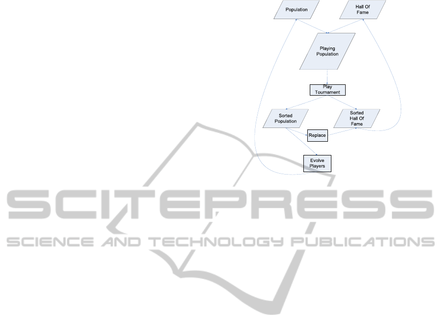
4.5.1 Halls of Fame
A hall of fame serves as a genetic memory for an evo-
lutionary system, and can be used as a benchmark of
previous generations. The hall of fame can be incor-
porated into the playing population as shown in figure
5.
Agents in the hall of fame are sterile; that is, there
are not used to create new agents. Their sole purpose
in the population is as a competitional benchmark for
the agents in the regular population. As long as the
regular agents are competing against the hall of fame
agents, their strategies should remember how to de-
feat the old strategies, and thus promote steady im-
provement.
The hall of fame begins with no agents included.
After the first tournaments are played, the agents that
are selected for reproduction are also inserted into the
hall of fame. In the next generation, the playing popu-
Figure 5: Selection and evolution using a hall of fame.
lation will consist of the regular population of agents,
as well as the hall of fame agents. Here, a decision
must be made. It is possible to create a very large
hall of fame, as memory permits, but this quickly be-
comes computationally expensive. Depending upon
how many agents are inserted into the hall of fame at
any given generation, the population size will increase
regularly. Given that many hands are required in each
tournament to eliminate all of the agents, as the pop-
ulation size grows, so too does the time required per
tournament, and hence, per generation.
Our hall of fame was capped, and could include
no more agents than were in the original population.
The best agents of previous generations would still be
present in the hall of fame, but the size of the hall
would not quickly get out of hand. Agents were re-
placed on a basis of futility. After each generation,
all agents in the total population would be evaluated,
including those agents in the hall of fame. Agents in
the entire population would be ranked according to
their performance, as per the previous selection func-
tion. Thus, if an agent was the last eliminated from
the tournament, it would receive a rank of 0, followed
by 1, etc., all the way down to the worst agents. The
REPLACE algorithm shows how agents in the hall of
fame are replaced every generation.
The Players and HallOfFame must be sorted
before calling REPLACE. numPlayersKept is the
amount of agents that are selected for reproduction
in a given generation. As long as the rank of the xth
best agent is lower than that of the appropriate hall of
fame member (i.e., the agent out-performed the hall
of fame member), the member is replaced. For exam-
ple, if the population and the hall of fame each contain
1000 members, and 100 agents are kept for reproduc-
tion every generation, then the rank of the 1st agent is
ICEC 2010 - International Conference on Evolutionary Computation
28

compared to the 900th hall of fame member. As long
as the agent out-performed the hall of fame member,
it will be added to the hall of fame. In the worst case,
when all agents in the hall of fame are replaced, the
hall of fame will still have a memory of 10 genera-
tions. The memory is generally much longer.
1: procedure REPLACE(HallOfFame[], hallSize, Players[],
numPlayersKept)
2: begin
3: j = 0;
4: for i = 0 to numPlayersKept - 1 do
5: if HallOfFame[hallSize-
numPlayersKept + i].OverallRanking() >
Players[j].OverallRanking() then
6: HallOfFame[hallSize - numPlayersKept +i] = Players[j++]
7: else continue
8: end if
9 end for
11: end REPLACE
Figure 6: Algorithm to replace the worst agents of the hall
of fame.
4.5.2 Co-evolution
(Lubberts and Miikkulainen, 2001; Pollack and Blair,
1998; Rosin, 1997) suggest the use of co-evolutionary
methods as a way of countering evolutionary forget-
ting. In co-evolution, several independant populations
are evolved simultaneously. Each population has its
own set of agents, and when reproduction occurs, the
eligible agents are chosen from the individual pop-
ulations. By evolving the populations separately, it
is hoped that each population will develop its own
strategies.
Multiple populations are created in the same way
as if there were only a single population. They are
then allowed to compete together, similarly to how the
agents can compete against agents in a hall of fame.
When it comes time for selection, agents are only
ranked against agents in their respective populations.
It is possible that one population may have a superior
strategy, and that the agents from this population out-
rank all agents from all other populations. Regardless,
agents are separated by population for evaluation and
evolution, in order to preserve any unique exploration
paths that alternate populations might be exploring.
Like halls of fame, the main strategy of co-
evolution is a deepening of the competition. By hav-
ing seperately evolving populations, the agents are
exposed to a more varied set of strategies, and thus
can produce more robust strategies. A single popula-
tion encourages exploration, but all strategies are ul-
timately derived similarly, and will share tendencies.
Although agents are only ranked against members of
their own population, they compete against members
of all of the populations, and as such, the highest rank-
ing agents are those that have robust strategies that
can defeat a wide variety of opponents.
Often, as co-evolution proceeds, a situation
known as an [arms race] will develop. In an arms-
race, one population develops a good strategy, which
is later supplanted by another population’s counter-
strategy. The counter-strategy is later replaced by an-
other counter-strategy, and so on. As each population
progresses, the global skill level also increases. By
creating multiple populations, an evolutionary strat-
egy develops that is less concerned with defeating
strategies that it has already seen, and more concerned
with defeating new strategies as they come along.
Halls of fame can be added to co-evolution. Our
system gives each population its own hall of fame,
with the same replacement strategy as when there is
only one population. As stated in section 4.5.1, the
goal of the halls of fame was to protect older strate-
gies that might get replaced in the population. In a co-
evolutionary environment, it is entirely possible that
one sub-population may become dominant for a pe-
riod of several generations. If a global hall of fame is
used, the strategies of the weaker populations would
quickly be replaced in the hall of fame by the strate-
gies of the superior population. Each population was
given its own hall of fame to preserve strategies that
might not be the strongest in the larger population,
but could still be useful competitive benchmarks for
the evolving agents.
4.5.3 Duplicate Tables
Poker is a game with a high degree of variance. Skill
plays a large part in the determination of which play-
ers will win regularly, but if a good player receives
poor cards, he will most likely not win. In (Billings,
2006), a method for evaluating agents is discussed,
which is modeled upon the real-world example of du-
plicate tables. In professional Bridge tournaments,
duplicate tables are used to attempt to remove some
of the randomness of the cards. Unfortunately, due
to the relatively high cost of performing duplicate ta-
bles at each hand, they are not used in the evolution
process. We only use duplicate tables after the evolu-
tion has been completed, as a method to test our best
evolved agents against certain benchmarks.
A duplicate table tournament is simply a col-
lection of smaller tournaments called single tourna-
ments. An agent sits at a table, just like they would
in a regular evaluation tournament. The tournament
is played until every agent at the table has been elim-
inated (i.e., every agent except one has lost all of its
chips). The rankings of the agents are noted, and the
next tournament can begin.
Unlike a normal tournament, where the deck
would be re-shuffled, and agents would again play to
elimination, the deck is reset to its original state, and
each agent is shifted one seat down the table. For ex-
ALGORITHMS FOR EVOLVING NO-LIMIT TEXAS HOLD'EM POKER PLAYING AGENTS
29

ample, if an agent was seated in position 5 at a table
for the first tournament, it will now be seated at posi-
tion 6. Likewise for all of the other agents, with the
agent formerly in position 9 now in position 0. Again,
the agents play to elimination. Since the deck was re-
set, the cards will be exactly the same as they were last
time; the only difference will be the betting strategies
of the agents. This method continues until each agent
has sat at each position at the table, and thus had a
chance with each possible set of hole cards.
After the completion of one revolution, the av-
erage ranking of the agents is calculated. A good
agent should be able to play well with good cards, and
not lose too much money with poor cards. It should
be noted that agents kept no memory of which cards
were dealt to which seats, nor which cards would be
coming as community cards. Each tournament was
played without knowledge of previous tournaments
being provided to the agents. After the completion
of a revolution and the noting of the rankings, the
agents would then begin a new revolution. For this
revolution, the deck is shuffled, so that new cards will
be seen. 100,000 such revolutions are played, and
the agents with the lowest average rankings are deter-
mined to be the best. In order for an agent to receive
a low ranking across all revolutions, it had to not only
take advantage of good cards and survive poor ones,
but it also had to take advantage of situations that its
opponents missed.
5 EXPERIMENTAL RESULTS
In order to evaluate agents, a number of benchmarks
were used. In (Beattie et al., 2007; Billings et al.,
2003; Booker, 2004; Schauenberg, 2006), several
static agents, which always play the same, regardless
of the situation, are used as benchmarks. These agents
are admittedly weak players, but are supplemented
by the best agents developed in (Beattie et al., 2007),
and can be used to evaluate the quality of our evolved
agents relative to each other. The benchmark agents
are as follow: Folder, Caller, and Raiser, that always
fold, call and raise, respectively, at every decision;
Random, that always makes random decisions; Cal-
lOrRaise, that calls and raises with equal likelihood;
OldBest, OldScratch, OldStart, that were developed
in (Beattie et al., 2007). OldScratch was evolved with
no head start to the evolution, OldBest was evolved
with a head start, and OldStart was given a head start,
but no evolution.
Baseline agents were evolved from a population
of 1000 agents, for 500 generations, playing 500
tournaments per generation. After each generation,
agents were ranked according to their average. Af-
ter each generation, the 100 best agents were selected
for reproduction, and the rest of the population was
filled with their offspring. LargeHOF agents were
also evolved from a population of 1000 agents, but
included a hall of fame of size 1000. SmallHOF
agents were evolved from a smaller population of 500
agents, with a hall of fame of size 500, and only
50 agents were selected for reproduction each gen-
eration. HOF2Pop agents were evolved using two
co-evolutionary populations of 500 agents each, each
with a hall of fame of 500 agents.
After 500 generations, the best agent from the
500th generation played 100,000 duplicate table tour-
naments, with each of the benchmark agents also sit-
ting at the tables. For each duplicate table tourna-
ment, each agent played in each possible seat at the
table, with the same seeds for the random numbers,
so that the skill of the agents, and not just the luck
of the cards, could be evaluated. After each duplicate
table tournament, the ranking of each agent at the ta-
ble was gathered, and the average was calculated after
the completion of all 100,000 duplicate table tourna-
ments. There were nine agents at the duplicate ta-
bles. The best possible rank was 1, corresponding
to an agent that wins every tournament, regardless of
cards or opponents. The worst possible rank was 9,
corresponding to an agent that was eliminated from
every tournament in last place. The results of our best
agents are shown in figure 7.
Figure 7 represents the results of the duplicate
table tournaments. In Figure 7, the Control agent
represtents the agent that is being evaluated, while
the other vertical bars represent the rankings of the
other agents in the evaluation of the control agent. For
example, the first bar of Random represents how the
Random agent performed against the Baseline agent,
the second bar represents how the Random agent per-
formed against the SmallHall agent, and so on.
The best results were obtained by the agents
evolved with a large hall of fame, but no co-evolution.
These agents obtained an average rank of 2.85 out of
9. Co-evolution seemed to have little effect upon the
agents when a hall of fame was used, and the agents
in the two co-evolutionary populations received aver-
age ranks of 2.92 and 2.93. The difference between
the best agents and the second best seems to be quite
small. A two-tailed paired t-test was conducted on
the null hypothesis thatthe ranks of any two distinct
agents were equal. In all cases, and for all exper-
iments, the null hypothesis was rejected with 99%
confidence. Although the difference is small, enough
hands were played that even small differences equate
to a difference in skill.
ICEC 2010 - International Conference on Evolutionary Computation
30

Random
Raiser
Folder
Caller
CallOrRaise
OldBest
OldScratch
OldStart
Control
0
1
2
3
4
5
6
7
8
9
10
Baseline
SmallHall
LargeHOF
HOF2Pop-1
HOF2Pop-2
Figure 7: Results of Duplicate Table Tournaments (Original
in Colour).
Although these agents were evolved separately,
they were able to develop strategies that were com-
petitive against each other. The small hall of fame
also seemed to have an impact; although the agent
was evolved in a smaller population than the baseline,
and thus had less competition, it was able to achieve a
rank of 3.48, which was more than one full rank better
than the baseline agent’s 4.73.
The baseline agent itself out-performed all of the
benchmarks, with the exception of the best agents
evolved in (Beattie et al., 2007), and the Folder. The
best agents evolved in our experiments out-ranked all
of the benchmarks, except for the folder, although the
best agents were much closer to the Folder’s rank than
the other agents. It was surprising that the Folder
performed so well, considering that it makes no de-
cisions, and simply lays down its cards at every deci-
sion point. However, in an environment where there
are many aggressive players, such as automatic raisers
and callers, many of these players will eliminate each
other early, giving better ranks to conservative play-
ers. The better ranks of our best agents tell us that
they can survive the over-active early hands until the
aggressive players are eliminated, and then succeed
against agents that actually make decisions.
6 CONCLUSIONS
Our algorithms present a new way of creating agents
for No-Limit Texas Hold’em Poker. Previous agents
have been concerned with the Limit variant of Texas
Hold’em, and have been centered around simulation
(Billings et al., 2002; Billings et al., 2003) and game
theoretical methods (Johanson, 2007; Schauenberg,
2006). Our approach is to evolve agents that learn
to play No-Limit Texas Hold’em through experience,
with good agents being rewarded, and poor agents be-
ing discarded. Evolutionary neural networks allow
good strategies to be discovered, without providing
much apriori knowledge of the game state. By mak-
ing minute changes to the networks, alternative solu-
tions are explored, and agents discover a guided path
through an enormous search space.
REFERENCES
Barone, L. and While, L. (1999). An adaptive learning
model for simplified poker using evolutionary algo-
rithms. In Angeline, P. J., Michalewicz, Z., Schoe-
nauer, M., Yao, X., and Zalzala, A., editors, Proceed-
ings of the Congress on Evolutionary Computation,
volume 1, pages 153–160, Mayflower Hotel, Wash-
ington D.C., USA. IEEE Press.
Beattie, B., Nicolai, G., Gerhard, D., and Hilderman, R. J.
(2007). Pattern classification in no-limit poker: A
head-start evolutionary approach. In Canadian Con-
ference on AI, pages 204–215.
Billings, D. (2006). Algorithms and Assessment in Com-
puter Poker. PhD thesis, University of Alberta.
Billings, D., Burch, N., Davidson, A., Holte, R., Schaeffer,
J., Schauenberg, T., and Szafron, D. (2003). Approxi-
mating game-theoretic optimal strategies for full-scale
poker. In Proceedings of the Eighteenth International
Joint Conference on Artificial Intelligence (IJCAI).
Billings, D., Davidson, A., Schaeffer, J., and Szafron, D.
(2002). The challenge of poker. Artificial Intelligence,
134(1-2):201–240.
Billings, D., Papp, D., Pena, L., Schaeffer, J., and Szafron,
D. (1999). Using selective-sampling simulations in
poker. In AAAI Spring Symposium on Search Tech-
niques for Problem Solving under Uncertainty and In-
complete Information.
Booker, L. R. (2004). A no limit texas hold’em poker play-
ing agent. Master’s thesis, University of London.
Campbell, M., Hoane, A. J., and hsiung Hsu, F. (2002).
Deep blue. Artificial Intelligence, 134:57–83.
Donninger, C. and Lorenz, U. (2005). The hydra project.
Xcell Journal, 53:94–97.
Hauptman, A. and Sipper, M. (2005). Gp-endchess: Using
genetic programming to evolve chess endgame play-
ers. In Keijzer, M., Tettamanzi, A., Collet, P., van
Hemert, J., and Tomassini, M., editors, Proceedings
of the 8th European Conference on Genetic Program-
ming.
Johanson, M. B. (2007). Robust stategies and counter-
strategies: Building a champion level computer poker
player. Master’s thesis, University of Alberta.
Kendall, G. and Whitwell, G. (2001). An evolutionary ap-
proach for the tuning of a chess evaluation function us-
ing population dynamics. In Proceedings of the 2001
IEEE Congress on Evolutionary Computation, pages
995–1002. IEEE Press.
ALGORITHMS FOR EVOLVING NO-LIMIT TEXAS HOLD'EM POKER PLAYING AGENTS
31

Lubberts, A. and Miikkulainen, R. (2001). Co-evolving
a go-playing neural network. In Proceedings of
the GECCO-01 Workshop on Coevolution: Turning
Adaptive Algorithms upon Themselves.
Pollack, J. B. and Blair, A. D. (1998). Co-evolution in the
successful learning of backgammon strategy. Mach.
Learn., 32(3):225–240.
Rosin, C. D. (1997). Coevolutionary Search among ad-
versaries. PhD thesis, University of California, San
Diego.
Samuel, A. L. (1959). Some studies in machine learning
using the game of checkers. IBM Journal of Research
and Development.
Schaeffer, J., Culberson, J., Treloar, N., Knight, B., Lu, P.,
and Szafron, D. (1992). A world championship caliber
checkers program. Artif. Intell., 53(2-3):273–289.
Schauenberg, T. (2006). Opponent modelling and search in
poker. Master’s thesis, University of Alberta.
Tesauro, G. (2002). Programming backgammon using self-
teaching neural nets. Artif. Intell., 134(1-2):181–199.
Thrun, S. (1995). Learning to play the game of chess. In
Tesauro, G., Touretzky, D., and Leen, T., editors, Ad-
vances in Neural Information Processing Systems 7,
pages 1069–1076. The MIT Press, Cambridge, MA.
ICEC 2010 - International Conference on Evolutionary Computation
32
