
MULTI-OBJECTIVE OPTIMIZATION OF BOTH PUMPING
ENERGY AND MAINTENANCE COSTS IN OIL PIPELINE
NETWORKS USING GENETIC ALGORITHMS
Ehsan Abbasi and Vahid Garousi
Software Quality Engineering Research Group, Department of Electrical and Computer Engineering
Schulich School of Engineering, University of Calgary, 2500 University Drive N.W. Calgary, Alberta, Canada
Keywords: Pump operation scheduling, Multi-objective genetic algorithm, Non-dominated sorting genetic algorithm,
Oil pipeline networks, Power optimization.
Abstract: This paper proposes an optimization model for the pipeline operation problem using a dual-objective non-
dominated sorting genetic algorithm (NSGA-II). One and foremost objective is to minimize pumping
energy costs. The second objective is to recognize the pipeline operators’ concern on pumps maintenance
costs by reducing the number of times pumps are turned on and off. This is commonly believed as a main
source of wear and tear on the pumps. The formulation of the problem is presented in detail and the model is
tested on a hypothetical case study (which is based on consultation with two industrial partners). The output
results are promising since they would give operators a better understanding of different optimal scenarios
on a “Pareto front”. Operators can visually assess several alternatives, and analyse the cost-effectiveness of
each scenario in terms of both objective functions.
1 INTRODUCTION
Oil is commonly transported using pipelines by the
propulsion from centrifugal pumps powered by
either electricity or gas. Pumps are located along the
pipelines at the approximate interval of 20 to 100
miles, depending on the geography and size of the
pipelines, and also capacity requirements. Finding
the optimal operation policy (regime) of oil pipelines
is challenging due to change prone energy cost
structures and complex hydraulic models that pose
distinct challenges to the optimization analysis
(Webb, 2007). The pipeline-operation optimization
problem is known as a mixed-integer non-linear
optimization problem due to constraints dictated by
pipelines non-linear hydraulic model (Lindell et al.,
1994).
Oil distribution systems consist of components
such as reservoirs, pipes, pump stations, and valves.
Pipes carry the fluid(s) from reservoirs to the
designated delivery points, e.g., refineries, or ports.
Pumps provide pressure needed to overcome gravity
and pipe friction. Valves are in charge of controlling
flows and pressures. The entire operation is
expensive, due to the fact that usually large masses
of fluid are to be pumped. However, significant
savings can be achieved through efficient energy
management, by matching pumping schedules with
time and shifting heavy pumping to periods with
cheap tariff rates (e.g., night time) (Webb, 2007).
The objective of a pumping optimization
problem is to provide the operator with the least-cost
operation policy for all pump stations in the pipeline
distribution system while maintaining the desired
delivery schedule. The operation policy for a set of
pumps is simply a schedule that indicates when a
particular (fixed-speed) pump or group of pumps
should be turned on or off over a specified period of
time, and the setting of the operating speed in case
of variable-speed pumps. The optimal policy
attempts to result in the lowest total operating cost
subject to a given set of boundary conditions and
system physical and operational constraints (Lindell
et al., 1994).
This paper proposes an optimization model based
on Non-dominated Sorting Genetic Algorithm
(NSGA-II) (Deb, 2001) for finding optimal pump
operation schedule. The two objective functions are:
(1) minimizing the cost of electric energy used by
pumps, and (2) minimizing the number of pump
on/off switching, which is a conventional surrogate
measure of pumps maintenance cost (Meetings mi-
153
Abbasi E. and Garousi V..
MULTI-OBJECTIVE OPTIMIZATION OF BOTH PUMPING ENERGY AND MAINTENANCE COSTS IN OIL PIPELINE NETWORKS USING GENETIC
ALGORITHMS.
DOI: 10.5220/0003063801530162
In Proceedings of the International Conference on Evolutionary Computation (ICEC-2010), pages 153-162
ISBN: 978-989-8425-31-7
Copyright
c
2010 SCITEPRESS (Science and Technology Publications, Lda.)

nutes, Spring and Fall 2009).
The final output of NSGA-II is a set of solutions
(known as a Pareto front or Pareto set) in which each
solution is better than the others in at least one of the
objective functions. The Pareto set could be used by
an operator to recognize the trade-offs of sacrificing
an objective in favour of another. For instance, in the
case of our problem, the operator can visually assess
the energy cost effectiveness obtained by several
extra pump switching. This way, he/she can make a
better decision on to whether toggle a pump status,
which causes wear on the unit, or operate the system
with a higher cost.
The remainder of the paper is outlined as
follows. Section 0 reviews the related works on the
problem of pump operation scheduling. The
mathematical definition of the objective functions
and constraints are thoroughly discussed in Section
0. Section 0 explains the basic concept of NSGA-II,
which is chosen as our solution methodology. The
model is applied to a hypothetical pipeline network
and the results are presented in Section 0. Sensitivity
analyses of the case study are discussed in Section 0.
Finally, Section 0 concludes the paper and discusses
some of our future works directions.
2 RELATED WORKS
The problem of pipeline operation optimization has
been a subject of study in three major areas: (1)
water distribution networks, (2) natural gas
transmission pipelines, and (3) oil products
transmission pipelines. Although each of these
networks has its own characteristics in terms of fluid
behaviour, contract terms, network size, structure
and elements, but the general idea that forms the
backbone of formulating these problems remains
similar.
In (Solanas and Montolio, 1987), dynamic
programming (DP) was used to evaluate the optimal
pumps operation scenario. However, for practical
distribution networks comprising more pump units
that should be evaluated in longer time frames,
application of dynamic programming (DP) needs
extensive computational resources due to the ‘curse
of dimensionality’. This problem limits the
application of all dynamic programming-based
techniques to large-sized networks.
Zessler and Shamir (Zessler and Shamir, 1989)
used the method of progressive optimality which is
an iterative DP. Jowitt and Germanopoulos has
proposed a method based on Linear Programming
(LP) in (Jowitt and Germanopoulos, 1992) and have
linearized the formulations. However, any
linearization of the formulations would lead to
linearization errors.
Lansey and Awumah have considered pump
switching as an additional constraint in their
optimization model in (Lansey and Awumah, 1994)
which accounts for the hardly-quantifiable
maintenance costs. They have adopted a two-level
approach which is compromised of a pre-
optimization level as well as the actual optimization
step.
Ulanicki et al. (Ulanicki et al., 2007) presented a
dynamic optimization approach to solve the optimal
pump scheduling problem. The model is claimed to
be faster than other existing approaches and follows
a two-stage approach in finding the solution.
Aligned with the trends of other optimization
problems, recent efforts are conducted to implement
the pump scheduling optimization using heuristic
and meta-heuristic approaches such as ant colony
(Ostfeld and Tubaltzev, 2008), particle swarm
(Wegley et al., 2000), or genetic algorithms (Ilich
and Simonovic, 1998).
In (Ostfeld and Tubaltzev, 2008), both design
and operation aspect of the pipeline system have
been modeled simultaneously in order to find the
optimal design of the network. In (Ilich and
Simonovic, 1998), a search within the feasible
region has been used which is claimed to improve
the efficiency in comparison with conventional
Genetic Algorithm (GA) method. The method has
been tested on a hypothetical network having five
serial pumps.
Zhang in (Zhang, 1999) couples GA with a
transient-hydraulic simulation model to generate and
evaluate trial pipe networks designs in search of an
optimal solution. The developed approach has been
applied to the New York City’s water supply
tunnels.
A great number of research works has also been
conducted for pipeline scheduling problem in the gas
pipelines sector. The problem was formulated with
GA and implemented in the Pascal programming
language by Goldberg in (Goldberg, 1987a) and
(Goldberg, 1987b). Wright and et al (Wright et al.,
1998) applied simulated annealing for finding the
optimum configuration and power settings for single
compressor problem as well as multiple compressors
arranged in series with constant pressure drops in the
segment. In (Betros et al., 2006), a genetic algorithm
is developed to optimize operation of gas pipeline
networks. Mora in (Mora, 2008) proposes a multi-
agent cooperative search technique to optimize the
operation of large and complex natural gas pipeline
ICEC 2010 - International Conference on Evolutionary Computation
154

networks.
Albeit oil pipeline stations are accounted as a
very important category of pipelines, but very few
research works have been devoted to this area. This
might be due to the fact that most of the research in
this area relates to corporate closed-source software
development projects which mostly do not appear in
publications and, ultimately prevents third parties
from analyzing or reusing the details of the solution
methods developed (SSI, Last Viewed: April 2010).
In (Veloso et al., 2004), a spreadsheet-based
computational tool was used to reduce the energy
consumption at each pumping station in oil
pipelines. Firstly, all possible pumping arrangements
are related to viable flow rates of the pipeline under
consideration. Then, a hydraulic simulator is used to
calculate the cost of each arrangement. All the cost
values are imported to a spreadsheet, which will be
used for selecting the minimum operation
arrangement by the operators as needed. This
method was applied to a 3 pipeline station network
and sounds memory and time intensive for larger
networks. Also, this “snap-shot” optimization
procedure does not guarantee that the set of pump
arrangements over a time period gives the minimum
cost. In (Abbasi and Garousi, 2010), a mixed-integer
linear formulation for finding optimal pump
operation schedule for oil pipelines is introduced.
The nonlinear equations have been linearized in
small operational flow rate ranges so that the
linearization errors are as marginal as possible. The
proposed formulation is capable of identifying the
most cost-effective solution to the linearized format
of the problem by giving the operation regime with
the lowest-cost energy consumption that satisfies the
mandatory operational and physical constraints
given a set of time-varying and quantity-varying
electricity tariffs. The formulation is then
implemented in the GAMS toolset and tested on a
hypothetical network.
This paper builds on top of the previous efforts
conducted in this area by considering multi-
objectives for the oil pipeline operation scheduling
problem which enables the operators to better
compare the cost effectiveness of the two objectives.
To the best of the authors’ knowledge, no existing
article has attempted considering these two
objectives at the same time.
3 MATHEMATICAL
FORMULATION
Implementation of any optimization problem calls
for a due assessment of the formulation constructing
the model. In this section, the pipeline operation
problem has been defined. The constraints and
objective functions of the problem have been
formulated and explained based on the relevant input
parameters and decision variables.
3.1 Problem Definition
The optimal operation of oil pipeline networks
involves selecting pumps’ operational schedules that
provide the least operational cost and also least
maintenance costs, while satisfying the system
constraints over a given finite time horizon. The key
components of the pump scheduling problem are
network hydraulics model, operational constraints,
and the objective functions.
3.2 Decision Variables
Depending on the system characteristics and time
window that the system is being modelled in, the
decision variables can vary in many forms. In the
case of this paper, the first set of decision variables
defined is the set of binary variables to indicate the
on/off status of the pumps at each time step.
The speed of the pump, in case of the variable-
speed pumps, is another decision variable.
3.3 The Two Objective Functions
The first objective function is to minimize the total
cost of electricity used by pumps in the whole
operation period. The second objective function is to
minimize the number of pumps switching (on to off,
or off to on) (Lindell et al., 1994). Each of these
objective functions is discussed and formulated next.
3.3.1 Objective Function 1: Minimization of
Total Electricity Cost used by Pumps
The most important objective function of the
pipeline operation scheduling problem represents the
total operating cost to be minimized. It is usually
comprised of energy cost for all of the pump units in
the whole operation period. Although other costs
such as penalties for deviation from the final
delivery contract might be considered, in this paper
the delivery contract has been considered as an
operational constraint of the system.
Pumping cost is evaluated based on the
electricity power tariff over the pumping duration.
Two types of electricity charging patterns are
usually used in the industry (Prindle, Last Viewed:
MULTI-OBJECTIVE OPTIMIZATION OF BOTH PUMPING ENERGY AND MAINTENANCE COSTS IN OIL
PIPELINE NETWORKS USING GENETIC ALGORITHMS
155
April 2010):
fixed electricity price rate;
time-variable or quantity-variable electricity
price rate;
Due to the fact that the latter case is more
general, this pricing pattern has been considered in
this paper.
Also, it has to be noted that the oil pipelines are
usually expanded over a reasonable geographical
area, and they usually enter into contracts with
several local electricity providers for their electricity
needs. In this context, oil pipeline operators face
various electricity purchasing contracts. Some
companies offer incentive prices for electricity usage
to sell more electricity while, on the other hand,
some others encourage their customers to consume
less electricity (Meetings minutes, Spring and Fall
2009).
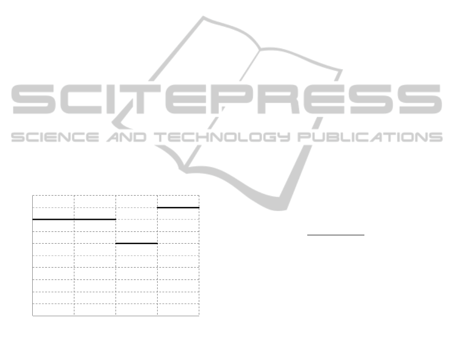
Some utilities encourage customers to limit their
consumption within a specific limit. Although any
nonlinear function of the consumed power and cost
is possible to be considered in GA models; however,
in this paper, it is considered that rate of electricity
follows the trend presented in Figure 1, which is a
generic case.
0
0.01
0.02
0.03
0.04
0.05
0.06
0.07
0.08
0.09
0.1
0 500 1000 1500 2000
ElectricityRate[$/kWh]
Power[kW]
Figure 1: Electricity Rates.
Power system companies are interested to have a
smooth load profile. This helps them in better
planning and scheduling of the power plants
operation to generate electricity by their highest
efficiency and also making use of the existing
transmission network close to nominal limit. Due to
these facts, usually power system providers consider
lower rates for the hours of the day that other
industrial sectors are off and lower consumption of
electricity is expected, which usually happens to be
around midnight.
In the case study reported in this paper, by
reviewing some example power contracts from our
industrial partner, it is assumed that the electricity
rate of daytime is twice the nighttime rate. It is
noteworthy that using genetic algorithm or any other
evolutionary algorithm as the solution technique,
any multiple segments and any type of cost
evaluation method could be modeled. Even any
nonlinear relationship between the electricity cost
rate and power consumption could be considered.
This is a significant feature of genetic algorithms
compared to more systematic approaches (e.g., LP,
MILP) on solving this problem which stems from
the flexibility of evolutionary algorithms in general.
Based on the aforementioned formulations, the
pumping cost objective function could be stated in
mathematical terms as:
t
i
J
j
t
i
t
i
PCost
11
)(min
(1)
In which, P
t
j
is the power consumed by pump j at
time step t and is a function of pumps pressure, flow
rate passing, its operating efficiency and the fluids
characteristic which is constant. Note that the full
list of mathematical notations defined and used in
this article can be found at the end of this article.
The following equation calculates the power
needed to operate the pump (Boulos et al., 2006):
i
t
i
t
i
t
i
PHQ
P
(2)
In the above equation, the terms flow, pressure
and efficiency are not independent. Technicians
usually consult empirically driven curves to find out
the operating status of a specific point. However, in
order to formulate the problem, an explicit
relationship between power and the other variables
is needed.
According to experiments conducted by
mechanical engineers (Boulos et al., 2006), the
power consumption of a pump could be determined
as a function of two independent variables of
pump’s speed and the flow rate of the fluid passing
by it. According to (Ulanicki et al., 2008), a
polynomial equation as stated in Equation (3) best
fits the empirically-extracted pump curves.
32 23t t tt tt t
ijjjjjjjjjj
P
aQ bQ scQ s ds
(3)
3.3.2 Objective Function 2: Minimization of
the Number of Pump State Changes
Another important cost issue that deserves conside-
ICEC 2010 - International Conference on Evolutionary Computation
156

ration is pump maintenance. An operation schedule
in which pumps are turned on and off very
frequently may reduce energy consumption;
however, this schedule may increase the wear and
tear on the pumps and increase the resulting pump
maintenance costs. It would also complicate the
operation of the system from the operator’s point of
view, i.e., the human operator has to constantly
review the operation schedule and turn the pumps on
and off. This task itself can be error prone and also
risky from system stability point of view.
The exact amount of maintenance costs is not
easily quantifiable, but it can be assumed that it
increases as the number of pump change status
increases. Hence, the number of pump change status
is used as a surrogate measure for the intangible
wear-and-tear maintenance costs. Therefore, the
switching objective is introduced into the model as
the second objective function. The operators can
then evaluate the trade-off of increasing cost to
reduce the number of switching by assessing the
model results.
This second objective function is formulated as
the following:
J
j
T
t
t
j
t
j
BpBp
1
1
1
1
min
(4)
In which, the absolute difference between the
binary variables associated with the status of a
specific pump in two successive time intervals is
summed up over the entire time horizon and for all
the pump units. The final result is the number of all
pumps status changes seen in the analysis period.
3.4 Constraints
The search space for pipeline scheduling problem, as
mentioned earlier, is confined by a number of
constraints. Based on the technical aspects, these
constraints can be divided into two categories: (1)
hydraulics constraints, and (2) operational
constraints.
The hydraulic-model constraints stem from
natural behaviour of a fluid being transported in a
pipeline. These constraints validate the feasibility of
the model in sense of the relationship between the
primary state variables of the hydraulic model.
On the other hand, the operational constraints
account for the tolerance of the equipments or in
concise, their operation limits, as well as the
constraints imposed by contracts or any other
external cause.
The mathematical equations representing the afo-
rementioned constrains are being discussed in the
next sub-sections.
3.4.1 Hydraulic Constraints
When assessing a particular pump-operating policy,
it is essential to make sure that the hydraulic state
variables of the model match their natural
connection couched in mathematical equations. Any
fluid movement in a pipeline network entails
satisfying the two fundamental laws of conservation
of mass and conservation of momentum (Mennon,
2005).
The conservation of mass law for non-
compressible fluids, as the name implies, states that
a balance exists between the summation of the
masses entering and exiting at any point on the
pipeline at a specific time instance. Equation (5):
tiQQ
t
Outi
t
Ini
,0
,,
(5)
The conservation of momentum which is based
on the conservation of energy law, establishes a
relationship between the pressure generation and
losses in the pipeline. For any two successive
pressure points, the differences in absolute head
(pressure) is equal to the net head added to the
system by pumps (if there’s any) minus the head lost
in either valves or segment’s friction loss due to the
movement of the fluid.
Difference in the altitude of the according
locations also contributes to the equation as static
heads. Equation (6) indicates the conservation of
momentum law (Mennon, 2005).
,
,
tt tt ttt
qq pp jjj
H
HS H HS PH PL V j t
p q nodes being connected by segment j
(6)
The term PL
t
j
is the pressure loss that occurs in
pipeline segment j at time instant t as a result of
friction which depends on the fluid type, pipeline
material and cross section, and the flow rate passing
the segment. This loss could be quantitatively
evaluated by the Darcy-Weisbach equation (Tullis,
1989) as follows:
tjQCLPL
t
jj
t
j
,
2
(7)
Since valves control high pressures, they appear
in Equation (6) accompanied by negative sign. The
last term of the Equation (6), PH
t
j
, represents the
pressure head added to the system by the pump
located on segment j at time t. The pumps head is a
function of the flow rate and also the speed of the
pump in case of variable speed pumps. The head-
MULTI-OBJECTIVE OPTIMIZATION OF BOTH PUMPING ENERGY AND MAINTENANCE COSTS IN OIL
PIPELINE NETWORKS USING GENETIC ALGORITHMS
157
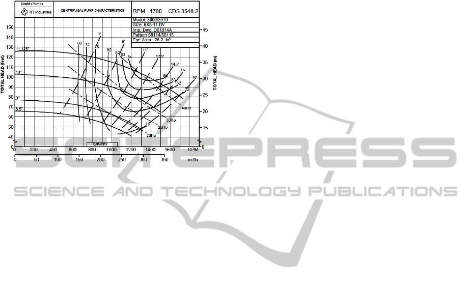
flow rate characteristic curve of a variable speed
pump is usually provided by the manufacturer for a
specific speed. A typical head/efficiency versus flow
rate curve of a variable-speed pump is presented in
Figure 2.
Figure 2: A typical head/efficiency versus flow rate curve.
Taken from (Goulds Pumps, Last Viewed: March 2010).
The head versus flow rate curve is often
approximated by a quadratic polynomial (Ulanicki et
al., 2008) as:
22
,
tt ttt
j j j j jj jj
P
HAPQBPQSCPS jt
(6)
3.4.2 Operational Constraints
Beside the basic hydraulic constraints that lay the
groundwork for implementing the model, a
multitude of operational constraints exist to propel
the solution towards an operational range. These
constraints generally originate from equipments’
operation limitations. Also, contract-related
constraints or environment-related constraints are
considered to fall in this category.
The pipeline wall is prone to cracks and leaks if
it is operated under high pressures. This not only
causes serious damages to the pipe but also, flow of
oil products to the environment causing
environmental damages which is followed by
considerable penalties. Hence, it is essential that the
operators keep the pressure of the nodes especially
on junctions lower than a threshold. On the other
hand, low pressure in the pipeline causes formation
of cavities in the fluid which causes corrosions on
the pipeline wall. More severely, these cavities form
a two phase flow, which seriously damages the
impellers of centrifugal pumps. The two mentioned
constraints are expressed in Equation (7).
tiHHH
Max
i
t
ii
,
min
(7)
Furthermore, the flow rate of the pipeline should
be bound to a certain limit, for high flow rates’
friction with pipeline wall causes overheat of the
pipe and product. This constraint is indicated by
Equation (8).
tjQQ
Max
j
t
j
,0
(8)
The speed of rotation of the pump units are
bounded by an upper and lower limit as stated by the
following equation:
tjBSSBS
t
j
Max
j
t
j
t
jj
,
min
(9)
Note that the binary variable B
t
j
sandwiches the
upper and lower bounds to zero at the times the
pump is off.
Finally, delivery contract imposes the most
prominent constraint on the problem. The pipeline
operator is supposed to deliver a contracted volume
of the product to the designated delivery points by
the end of the planning time period. Hence, the
summation of the volume of the fluid being
delivered to specified locations in every time step
should be more than or equal to the contracted
amount for that specific location. The corresponding
equation to this constraint is as follows:
iConQSink
T
t
i
t
i
1
(10)
4 SOLUTION METHODOLOGY
The Fast Non-dominated Sorting Genetic Algorithm
(NSGA-II) is a very popular approach in MOGA, as
it has been used in many existing works such as
(Kang et al., 2009) and (Baran et al., 2005). Thus, it
was also chosen to be used in this work. Efficient
sorting and ability to maintain a diverse set of elite
population could be counted as features of NSGA-II
(Deb, 2001).
5 CASE STUDY
To evaluate our optimization technique, we are
working with a Western Canadian oil pipeline
operator to apply our optimization technique to its
pipeline network. However, as of this writing,
extraction of actual parameters to be able to execute
the algorithm has not been completed yet.
In the mean-time, we evaluate the proposed ap-
proach on a hypothetical oil distribution system
comprising of 5 pipeline segments which connect 6
ICEC 2010 - International Conference on Evolutionary Computation
158
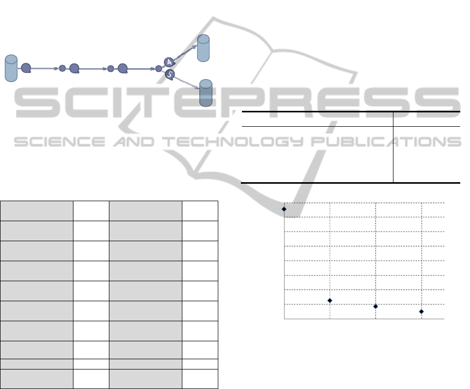
nodes. The system is designed to feed two delivery
nodes from a single source on a dendritic structure.
All of the segments are equipped with pump units
and valves. Structure of the network is shown in
Figure 3. It has been assumed that the whole
assessment timeframe is one day comprising three
time-of-use electricity tariffs, in which the cost of
the last time period is half of the cost of the other
two. The parameters of this hypothetical test system
could be found in the Table 1. The formulation of
this hypothetical system results in 62 decision
variables and 48 constraints.
1
2
3
1
2
Figure 3: Configuration of the test case pipeline network.
It should be noted that the formulation structure
is generic and any number of sources and delivery
points and also branches could be considered easily.
Table 1: Parameters of the hypothetical test system.
j
CL
0.3
min
j
S
0.2
i
Con
i=4,5
60
Max
j
S
2.5
min
i
H
300
j
AP
2.3×10
-6
Max
i
H
1000
j
BP
8.3
Max
j
Q
100
j
CP
4.6×10
-3
j
a
7.4×10
-3
j
c
5.7×10
-7
j
b
1.66
j
d
3.6×10
-3
i
SH
0
Electricity Rate 1 0.08
Electricity Rate 2 0.06 Electricity Rate 3 0.09
Change Rate
Value 1
1000
Change Rate
Value 2
1500
In order to investigate the ability of NSGA-II
dealing with pipeline operation optimization
problem, a MATLAB program was developed. The
GA parameters set for the algorithm is presented in
Table 2. These parameters were empirically
calibrated and were found as suitable parameters
after a series of experimental runs, using ideas from
the work of (Garousi, 2008).
By running the MATLAB program in MATLAB
version 2009a, the Pareto front depicted in Figure 4
was generated. Due to the random effects of GA, we
executed the MATLAB program for 50 times and
the average execution time of each run on a PC with
Windows Vista, a 2.30 GHz CPU, and 2 GB of
RAM was 885.36 seconds (about 15 minutes).
As it could be seen from the Pareto, higher cost
of operation comes with zero switching while the
case with three switching is the operation scenario
with the lowest cost. Noteworthy, the amount of
operation cost reduction is reasonable between
having one switching and no switching state. Also,
this amount is not negligible between having one
switching and two switching while no reasonable
cost reduction is achieved for the case of three pump
switching. Pipeline operators can make decisions
based on such Pareto to visually identify the trade-
offs of operations with low costs.
Table 2: Calibration of GA parameters.
Parameter Value
Population size 315
Number of Generations 100
Crossover Rate 80%
Mutation selection strategy Gaussian
164
166
168
170
172
174
176
178
180
0123
OperationCost[$]
X1000
PumpSwitching
Figure 4: Four solutions on the optimal Pareto-front of the
test case problem.
Table 3 and 4 present detailed output data
(decision variables) for two of the four pump
operation regimes. It should be noted that the
pressure reduction by valves of the network are
managed to be zero in all combinations. The first
pump is always running in order to add enough
pressure to compensate for the loss of the first line
segment. Similarly the second pump is always ON to
add enough pressure for the fluid to pass through the
pipeline.
MULTI-OBJECTIVE OPTIMIZATION OF BOTH PUMPING ENERGY AND MAINTENANCE COSTS IN OIL
PIPELINE NETWORKS USING GENETIC ALGORITHMS
159
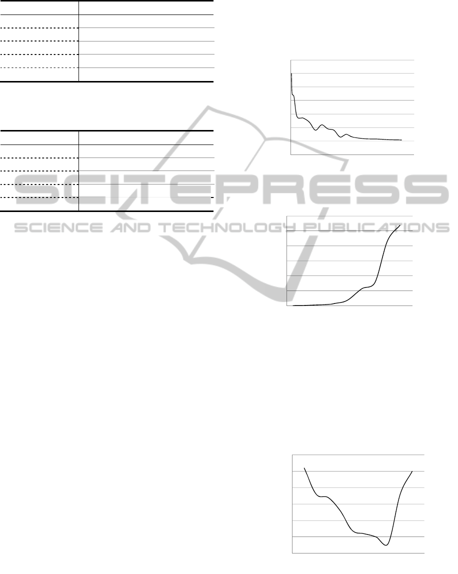
Table 3: The pump operation schedule (speed values) for
zero switching.
Pump Period 1 Period 2 Period 3
1 2.4 2.4 2.4
2 1.7 1.7 1.7
3 0 0 0
4 0 0 0
5 0 0 0
* Operation Cost = $179,110.00
Table 4: The pump operation schedule (speed values) for
one switching.
Pump Period 1 Period 2 Period 3
1 2.4 2.4 2.4
2 0.9 0.9 0.77
3 0 0 0.43
4 0 0 0
5 0 0 0
* Operation Cost = $166,500.00
6 SENSITIVITY ANALYSIS
In order to assess the effect of variation of GA
parameters on the performance of the model, several
sensitivity analyses were conducted, as discussed
next.
6.1 Population Size
The population size of the solutions has been
changed from 10 to 500 in the increments of 50. The
optimization results for the amount of cost for the
second objective of 3 switching have been presented
in Figure 5.
As it could be seen from Figure 5, the more the
size of the population grows, less improvement in
the cost is seen due to the fact that the GA results get
closer to the global optimum which may not be
improved then after. Hence, the effect of population
growth beyond 400is more or less subtle.
Expectedly, the execution time increases
dramatically as population size is incremented. The
variation of execution time versus the population
size is presented in Figure 6. Inspecting Figure 5 and
Figure 6 simultaneously, it is clear that any
increment in population size after the margin of 300
causes slight improvement in operation cost but with
tremendous increase in execution time. For instance,
shifting from population size of 300 to 900 leads to
0.04% improve in operation cost of the solution with
three switching but the execution time of 900
population is approximately 84.4 times longer than
that of 300. This poses another factor in selecting the
right population size for the algorithm which is the
trade-off in cost improvement and the raise in
execution time.
164.8
164.9
165
165.1
165.2
165.3
165.4
165.5
0 200 400 600 800 1000
OperationCost[$]
X1000
PopulationSize
Figure 5: Decrease in cost of operation versus increase in
GA’s population size setting.
0
5
10
15
20
25
30
0 200 400 600 800 1000
ExeutionTime[hours]
PopulationSize
Figure 6: Execution time versus population size.
6.2 Crossover Rate
Figure 7 depicts the variation of the cost of operation
of three switching for different values of the GA
crossover rate. This empirical analysis justifies the
choice of the crossover rate of 80% since the best
result is achieved at this point.
164.95
165
165.05
165.1
165.15
165.2
165.25
0 0.2 0.4 0.6 0.8 1
OperationCost[$]
X1000
CrossoverRate
Figure 7: Minimal cost of operation found for 3 switching
versus crossover rate.
ICEC 2010 - International Conference on Evolutionary Computation
160

7 CONCLUSIONS AND FUTURE
WORKS
In this work, an optimization model was developed
for minimizing the costs of pumping while satisfying
fluid flowing and hydraulic constraints. Several
major difficulties including complicated electrical
tariffs, wear and tear of the pipelines has been
implicitly considered. Multi-objective genetic
algorithm was chosen as the optimization technique.
This technique can help the operators to choose the
appropriate operating point based on their
experience and unformulated priorities considering
both objective functions values. The numerical
results indicate the viability and applicability of the
model.
As future work directions, we plan to work with
our industrial partner, Pembina Pipelines, a Western
Canadian oil pipeline operator, to apply our
technique to their pipeline networks and to optimize
their operational costs. Also, we intend to make use
of the flexibility of GA to formulate the multi-
products pipelines operation. This problem is
challenging due to the fact that the movement of
various liquids that are being transported
simultaneously by the pipeline should be modelled
over the time span.
ACKNOWLEDGEMENTS
This work was supported by the Alberta Ingenuity
New Faculty Award grant number 200600673. We
would like to thank Pembina Pipeline Corporation
for its collaborations in this project.
REFERENCES
Abbasi, E. & Garousi, V. (2010) Decreasing The Carbon
Footprint Of Oil Pipelines By Minimizing Pumping
Costs Using Milp. Informs Optimization Society
Conference On Energy, Sustainability And Climate
Change (Cescc). Gainesville, Florida, Usa.
Baran, B., Lucken, C. & Sotelo, A. (2005) Multi-
Objective Pump Scheduling Optimizatoin Using
Evolutionary Strategies. Advances In Engineering
Software, 36, 39-47.
Betros, K. K., Sennhauser, D., Jungowski, J. & Golshan,
H. (2006) Large Pipeline Networks Optimization -
Summary And Conclusion Of Transcanada Research
Effort. International Pipeline Conference. Calgary,
Canada, Asme.
Boulos, P. F., Lansey, K. E. & Karney, B. W. (2006)
Comprehensive Water Distribution Systems Analysis
Handbook For Engineers And Planners, Pasadena,
California, Mwh Soft.
Deb, K. (2001) Multi-Objective Optimization Using
Evolutionary Algorithm, New York, Ny, Usa, John
Wiley & Sons Inc.
Garousi, V. (2008) Empirical Analysis Of A Genetic
Algorithm-Based Stress Test Technique For
Distributed Real-Time Systems. Genetic And
Evolutionary Computation Conference (Gecco).
Atlanta, Georgia, Usa.
Goldberg, D. E. (1987a) Computer-Aided Pipeline
Operation Using Genetic Algorithms And Rule
Learning. Part I: Genetic Algorithms In Pipeline
Optimization. Engineering With Computers, 3, 35-45.
Goldberg, D. E. (1987b) Computer-Aided Pipeline
Operation Using Genetic Algorithms And Rule
Learning. Part Ii: Rule Learning Control of A Pipeline
Under Normal and Abnormal Conditions. Engineering
With Computers, 3, 47-58.
Goulds Pumps (Last Viewed: March 2010)
Http://Www.Gouldspumps.Com/Download_Files/391
0/35482.Pdf.
Ilich, N. & Simonovic, S. P. (1998) Evolutionary
Algorithm For Minimuzation of Pumping Cost.
Journal of Computing In Civil Engineering, 12, 9.
Jowitt, P. W. & Germanopoulos, G. (1992) Optimal Pump
Scheduling In Water Supply Networks. Journal Of
Water Resources Planning And Management, 118, 17.
Kang, Y. H., Zhang, Z. & Huang, W. (2009)
Nsga-Ii Algorithms For Multi-Objective Short-Term
Hydrothermal Scheduling Power And Energy
Engineering Conference, Appeec. Asia-Pacific.
Lansey, K. E. & Awumah, K. (1994) Optimzal Pump
Operations Considering Pump Switches. Journal Of
Water Resources Planning And Management, 120, 19.
Lindell, E., Ormsbee, K. & Lansey, E. (1994) Optimal
Control of Water Supply Pumping Systems. Journal of
Water Resources Planning And Management, 120,
237-252.
Meetings Minutes (Spring And Fall 2009) Meetings
Between The University Of Calgary's Softqual
Research Team And Pembina Pipeline Staff.
Mennon, E. S.
(2005) Piping Calculation Manual, New
York, Mcgraw-Hill.
Mora, T. E. (2008) Optimization Of Pipeline Operations
Using Biologically-Inspired Computationsal Models.
Department of Electrical And Computer Engineering.
Univarsity of Calgary.
Ostfeld, A. & Tubaltzev, A. (2008) Ant Colony
Optimization For Least-Cost Design And Operation
Of Pumping Water Distribution Systems. Journal Of
Water Resources Planning And Management, 134,
107-118.
Prindle, W. (Last Viewed: April 2010) Customer
Incentives For Energy Efficiency Through Electric
And Natural Gas Rate Design. National Action Plan
For Energy Efficiency, 2009. Http://Www.Epa.Gov/
Rdee/Documents/Rate_Design.Pdf.
Solanas, J. L. & Montolio, J. M. (1987) The Optimum
Operation Of Water Systems International Conference
MULTI-OBJECTIVE OPTIMIZATION OF BOTH PUMPING ENERGY AND MAINTENANCE COSTS IN OIL
PIPELINE NETWORKS USING GENETIC ALGORITHMS
161

On Computer Applications For Water Supply And
Distribution. Leicester, England.
Ssi (Last Viewed: April 2010) Ssi Scheduling.
Http://Www.Ssischeduling.Com/.
Tullis, J. P. (1989) Hydraulics Of Pipelines: Pumps,
Valves, Cavitation, Transients, Wiley-Interscience.
Ulanicki, B., Kahler, J. & Coulbeck, B. (2008) Modeling
The Efficiency And Power Characteristics Of A Pump
Group. Journal of Water Resources Planning And
Management, 134, 88-93.
Ulanicki, B., Kahler, J. & See, H. (2007) Dynamic
Optimization Approach For Solving An Optimal
Scheduling Problem In Water Distribution Systems.
Journal of Water Resources Planning And
Management, 133, 10.
Veloso, B. C., Pires, L. F. G. & Azevedo, L. F. A. (2004)
Optimization Of Pump Energy Consumption In Oil
Poipelines. International Pipeline Conference.
Calgary, Canada, Asme.
Webb, K. (2007) Non-Chronological Pipeline Analysis
For Batched Operations. Psig Annual Meeting.
Calgary, Alberta.
Wegley, C., Eusuff, M. & Lansey, K. (2000) Determining
Pump Operations Using Particle Swarm Optimization.
Joint Conference On Water Resource Engineering And
Water Resources Planning And Management.
Minneapolis, Minnesota, Usa.
Wright, S., Somani, M. & Ditzel, C. (1998) Compressor
Station Optimization. Denver, Usa, Pipeline
Simulation Interest Group.
Zessler, U. & Shamir, U. (1989) Optimal Operation of
Water Distribution Syatems. Journal of Water
Resources Planning And Management, 115, 18.
Zhang, Z. (1999) Fluid Transients And Pipeline
Optimization Using Genetic Algorithms. Graduate
Department of Civil And Environment Engineering.
University Of Toronto, Master's Thesis.
LIST OF NOTATIONS
t
j
B
Binary variable that indicates the status of the
pump on segment j at time t
j
CL The constant term of the Darcy-Weisbach equation
for segment j
i
Con Contracted volume of fluid that should be
transported in the time frame to the delivery point
located on node i
()
t
j
Cost
Operation cost function associated with pump j
at time t
t
i
H
Average pressure head associated with node i at
time t
min
i
H Minimum acceptable head of node i
Max
i
H
Maximum acceptable head of node i
t
j
P Power consumed by pump j at time t
t
j
PH
Head added to the network by pump j at time t
t
j
PL Pressure loss of segment j at time t
t
j
Q Average flow rate associated with pipeline
segment j at time t
Max
j
Q Maximum acceptable flow rate of segment j
t
Ini
Q
,
Summation of the flow entering node i at time t
t
Outi
Q
,
Summation of the flow exiting node i at time t
t
j
S Ratio of the speed of the pump on segment j at
time t to its nominal speed
min
j
S Minimum ratio of the speed of the pump on
segment j to its nominal speed
Max
j
S Maximum ratio of the speed of the pump on
segment j to its nominal speed
i
SH Static head associated with node i
t
j
V Valve pressure drop of segment j at time t
j
AP First coefficient of the head versus flow and speed
equation of the pump on segment j
j
BP
Second coefficient of the head versus flow and
speed equation of the pump on segment j
j
CP Third coefficient of the head versus flow and
speed equation of the pump on segment j
j
a First coefficient of the power versus flow and
speed equation of the pump on segment j
j
b Second coefficient of the power versus flow and
speed equation of the pump on segment j
j
c Third coefficient of the power versus flow and
speed equation of the pump on segment j
j
d Fourth coefficient of the power versus flow and
speed equation of the pump on segment j
The constant term of the power versus flow,
efficiency and head equation
ICEC 2010 - International Conference on Evolutionary Computation
162
