
COLLECTIVE BEHAVIOUR IN INTERNET
Tendency Analysis of the Frequency of User Web Queries
Joan Codina-Filba and David F. Nettleton
Technology Department, Pompeu Fabra University, Tanger 122-140, Barcelona, Spain
Keywords: Internet user search query, User collective behaviour, Google Trends, Machine learning techniques,
Classification, Tendency.
Abstract: In this paper we propose a classification for different observable trends over time for user web queries. The
focus is on the identification of general collective trends, based on search query keywords, of the user
community in Internet and how they behave over a given time period. We give some representative
examples of real search queries and their tendencies. From these examples we define a set of descriptive
features which can be used as inputs for data modelling. Then we use a selection of non supervised
(clustering) and supervised modelling techniques to classify the trends. The results show that it is relatively
easy to classify the basic hypothetical trends we have defined, and we identify which of the chosen learning
techniques are best able to model the data. However, the presence of more complex, noisy or mixed trends
make the classification more difficult.
1 INTRODUCTION
Collective user behaviour has been studied from a
sociological point of view, and different models
have been defined for how people follow fashion
trends, demonstrate „herd instinct‟, and so on. In
terms of Internet search, there is not so much
investigative work in the field, hence the motivation
for the present study, although from a marketing
viewpoint it is studied intensively, using basic
statistical gathering and analysis.
When measuring the impact of an event or a
marketing campaign for a given population, surveys
are usually performed at one point in time as it is
very difficult and expensive to repeat this
measurement periodically with a set of sufficiently
balanced respondents. A time-series survey needs to
be designed and commenced before the event, and
maybe the questionnaire is not adequately designed
to measure some unexpected response of the
population or the influence of external events.
Google Trends offers up to six years of weekly data
for the most popular words in user queries, allowing
the study of temporal market evolution and response
to events, a new opportunity that was not measurable
in the past.
In this paper the objectives are as follows: we
use a program for which an enhanced version has
recently become publicly available, (Google Trends,
2010), to download frequency statistics over time of
specific search keywords. We define a hypothetical
classification for some key tendencies which can be
seen over time for user search frequencies, giving a
set of real examples. We define a set of features
which describe the data, and which can be used as
input variables. Then we test several different
supervised learning techniques as classifiers for each
of the reference trends we have defined. We also
process the data using a non-supervised (clustering)
technique. We define four reference trends: (A)
Phenomenon or steady increase/decrease over whole
time period considered; (B) Specific bursts; (C)
Singular surge of interest; (D) Periodic variation.
We find it is relatively easy to classify the basic
hypothetical trends we have defined, although the
precision is of course very dependent on the clarity
of the examples chosen for the train and test
datasets. The scope and orientation of the current
work is limited to the definition and classification of
a carefully selected representative set of trends.
Other possibilities, such as prediction, alternatives
for data representation and datasets, and inter-trend
comparisons are reserved for future work.
The paper is structured as follows: in Section 2
we look at related work, state of the art, and give
some background to the social context of collective
168
Codina-Filba J. and Nettleton D..
COLLECTIVE BEHAVIOUR IN INTERNET - Tendency Analysis of the Frequency of User Web Queries.
DOI: 10.5220/0003069501680175
In Proceedings of the International Conference on Knowledge Discovery and Information Retrieval (KDIR-2010), pages 168-175
ISBN: 978-989-8425-28-7
Copyright
c
2010 SCITEPRESS (Science and Technology Publications, Lda.)

behaviour in general; in Section 3 we define some
specific examples from Google Trends; in Section 4
we explain the factors we have derived to represent
the data; in Section 5 we present the data modelling
techniques used; in Section 6 we explain the
experimental setup and present the classifier and
clustering results; finally, in Section 7 we make
some conclusions about the current work.
2 RELATED WORK
A recent book (Surowiecki, 2005) called “The
Wisdom of Crowds" has become “cult” reading for
Internet marketers. One of its hypotheses is that
sometimes, the majority “know best”. In (Klienberg,
2002), on the other hand, it is proposed that the
nature of user access stabilizes until a given event or
press release in the media (information stream),
provokes a “burst” of interest in a determined topic,
web site or document. (Aizen, 2003) introduces the
concept of “batting average”, which implies that the
proportion of visits that lead to acquisitions is a
measure of an item's popularity. The authors
illustrate its usefulness as a complement to
traditional measures such as visit or acquisition
counts alone. Their study is in the context of movie
and audio downloads in e-commerce sites. They use
a stochastic modelling framework of hidden Markov
models (HMMs) (Rabiner, 1989) to explicitly
represent the underlying download probability as a
“hidden state” in the process, and identifying the
moments when this state changes. Access to specific
documents is also modelled as a function of time.
The study of Internet search queries with a high
frequency is often motivated by the need for the
caching of results by search engine providers. One
such study is that of (Silvestri, 2004), in which hit-
ratio statistics were calculated for different
replacement policies and 'prefetching', to identify an
optimum policy.
On the other hand, there have been different
studies to identify which are the most popular terms
in general used in queries to search engines. The
frequencies are typically summed for a given period
of time. In (Baeza, 2005) the top 10 query terms and
queries were identified for the Chilean TodoCL
search engine. The top 10 queries for this search
engine were cited as being, in descending order of
frequency: {chile, sale, cars, santiago, radios, used,
house, photos, rent, Chilean}. Although this is useful
for the search engine provider to know, it does not
tell us about any trends or changes over time.
(Cacheda, 2001) made a similar study of the BIWE
search engine, and gave the most popular search
terms, such as the following: {sex, free, photos,
mp3, chat, famous} in descending order of
frequency.
Other studies have focussed more from the point
of view of the most popular documents returned by a
query, rather than the popularity of the query terms
themselves, although the two are clearly inter-
related. In (Cho, 2000) it was proposed that the
evolution of the popularity of content pages in
Google search results was influenced by the Page
Rank algorithm itself. It was stated that this is
because most of the user traffic is directed to popular
pages under a search-engine dominant model. The
plot of popularity against time showed a relatively
long period of low frequency followed by an abrupt
increase to a maximum value.
With reference to the application of different
unsupervised learning methods to web log analysis,
in (Nettleton and Baeza, 2008) a web log from the
TodoCL search engine was processed by different
clustering techniques (Fuzzy c-Means, Kohonen and
k-Means). A consensus operator was used to choose
the best predicted category/cluster by majority vote.
The objective was to group similar queries, based on
query search characteristics such as hold times,
ranking of the results clicked, and so on.
The identification of trends in Internet, such as the
top 10 queries by frequency, calculated on a weekly
basis, or the most popular web pages, is already an
area of great interest for the search engine
companies, due to commercial interests. „Google
Trends‟ (Google Trends, 2010) is an application
useful for observing tendencies of the frequency of
user query key words over time. Recently, Google
has made the raw data available to users, which can
be downloaded in an Excel file. This can be
subsequently processed by different statistical
techniques. In the literature, there are several recent
references of academic studies using „Google
Trends‟. For example, (Choi, and Varian, 2010) try
predicting curve trends for the automotive industry
using statistical regression model techniques. Also
(Choi and Varian, 2009) apply similar techniques to
the prediction of initial claims for unemployment
benefits in the U.S. welfare system. In (Rech, 2007),
„Google Trends‟ is used for knowledge discovery
with an application to software engineering.
COLLECTIVE BEHAVIOUR IN INTERNET - Tendency Analysis of the Frequency of User Web Queries
169
3 EXAMPLES FROM GOOGLE
TRENDS – RELATING
COLLECTIVE USER SEARCH
BEHAVIOUR TO SPECIFIC
TENDENCIES
In Section 3.1 we define four hypothetical collective
behaviour trends for the popularity of Internet search
terms. Then in Section 3.2 we illustrate each
hypothetical trend with real examples. The query
examples of Section 3.2 are taken from Google
Trends: http://google.com/trends. We have
downloaded the raw data into an Excel file, using
the corresponding option provided by Google
Trends, and have produced the graphics in Excel.
3.1 Categories of Collective Behaviour
–Internet Search Trends over Time
We will now define four basic collective behaviour
categories which can be identified as frequency
trends over a period of time. Then in Section 3.2 we
will relate them to four representative examples
from Google Trends.
A. Phenomenon. Steady and solid increase or
decrease exhibited over all the time period studied.
B. Specific bursts of increase/decrease which can
be identified with specific campaigns or news/press
releases. B.1. Idem as B, with the difference that the
frequency level after burst keeps constant at a higher
level than previous to the burst.
C. Surge of interest concentrated over a highly
defined and limited time period (usually short).
Frequency level after surge returns to original level.
D. Periodic Variation (increase or decrease)
identifiable with season/time of calendar year (for
example, Christmas).
3.2 Query Trend Examples
In the following Section we illustrate plots of trends
of specific queries generated in Excel using data
exported from „Google Trends‟. In each case we
classify the trend using the principal tendency, but
which can also manifest as secondary trends, one or
more of the category types defined in Section 3.1.
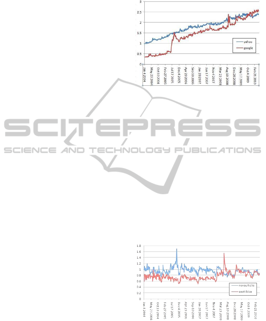
3.2.1 Principal Tendency Type A
Search Terms “yahoo”, “google”. With reference
to Figure 1, we observe an example of principal
tendency type A and secondary type B.1. The
Figure 1: Plot of frequency Vs time for the use of “yahoo”
and “google” as search terms.
graphic shows a phenomenon of overall increase in
interest for both search terms over the six year
period shown, with „yahoo‟ having a general
advantage over „google‟. Type B.1 burst displayed
by „google‟ during 3
rd
quarter of 2005, momentarily
exceeding „yahoo‟, after which „google‟ drops once
again below „yahoo‟ but remains at a higher level
than previous to the burst.
3.2.2 Principal Tendency Types B, A
Search terms “renault clio”, “seat ibiza”. In
Figure 2 we see examples of principal tendency type
B and secondary tendency type D. Both
brand/models are on the same track until mid 2005
when “renault clio” established a clear lead, “seat
ibiza” recovering the lead two years later (June
2008). We observe seasonal and ad-hoc variations
with two major ad-hoc spikes for both search terms
with drops in November/beginning of December.
Figure 2: Plot of frequency Vs time for the use of “renault
clio” and “seat ibiza” as search terms.
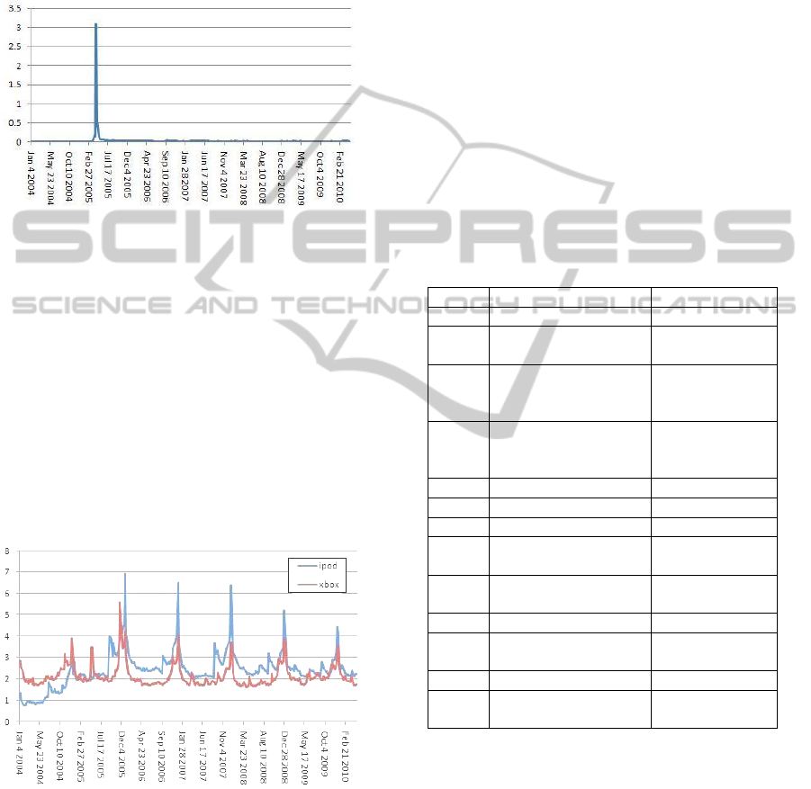
3.2.3 Principal Tendency Type C
Search term “ratzinger”. In Figure 3 we see a clear
example of principal tendency type C, representing a
KDIR 2010 - International Conference on Knowledge Discovery and Information Retrieval
170
sporadic burst. It manifests a very highly defined
interest in a limited time period corresponding to a
specific point in time (the election of the new Pope),
with posterior fall to original level. However, we
could study the post-burst frequencies on a higher
resolution scale to detect any smaller posterior
variations.
Figure 3: Plot of frequency Vs time for the use of
“ratzinger” as a search term.
3.2.4 Principal Tendency Type D
Search Terms “ipod”, “xbox”. With reference to
Figure 4, we observe an example of principal
tendency type D and secondary type B. The seasonal
tendencies and campaigns are clearly seen from
December 2005 onwards, with peaks over the
Christmas period especially for three years 2005-
2007 (both ipod and xbox). Also there are some
spikes related to specific commercial
campaigns/launches (tendency type B): new xbox
launched in May 2005, and the Apple Itunes/Ipod
launch in September 2005.
Figure 4: Plot of frequency Vs time for the use of “ipod”
and “xbox” as search terms.
We plotted and analysed each of the other search
terms used as examples for each tendency type (see
Table 2 in Section 6), but the plots and analyses are
not shown here for the sake of brevity.
4 DERIVED FACTORS USED
FOR DATA REPRESENTATION
We have derived a set of 13 factors for representing
the trends, which are to be used as inputs to the data
modelling techniques. The factors are listed in Table
1. We observe that factors 1 to 4 and 11 to 14 refer
to the features, whereas factors 5 to 10 refer to the
time period as a whole. In this way, we use average
values, standard deviations and ratios to capture the
characteristics, which differ significantly between
tendencies A, B, C and D. It is important to note that
all the data values were normalized before creating
the train/test folds for data modelling. The
normalized value is in the range between 0.0 and
1.0, calculated by dividing by the maximum value
for the corresponding variable (not min-max because
for our dataset the minimum value of all variables is
always zero).
Table 1: Defined factors used for data modelling.
Factor
Description*
Example (ipod)
1
Number of features
8
2
Average distance
between features
0.139
3
Standard deviation
distance between
features
0.04
4
Average ratio „y‟
after feature / „y‟
before feature
1.1
5
„y‟ at start of trend
0.143
6
„y‟ at end of trend
0.325
7
„y‟ at middle of trend
0.357
8
„y‟ at start of trend /
„y‟ at end of trend
0.44
9
Standard Deviation
„y‟
0.12
10
Average „y‟
0.35
11
Average feature
height
0.384
12
Average feature base
0.677
13
Average ratio height /
base
5.67
*The „y‟ value represents the frequency of the query term, that is,
the y-axis value of Figures 1 to 4.
With reference to Figure 4 and Table 1, we observe
the trend of the query term „ipod‟ and the
corresponding derived factors for that trend. For
„ipod‟, the first factor (1) „number of features‟ is
defined as 8, and we observe in Figure 4 that from
December 2005 there are five well defined periodic
features consistent with our tendency type D.
However, previous to December 2005, there are 3
features (smaller peaks) for „ipod‟ which are less
periodical and more „ad-hoc. This is the part of the
COLLECTIVE BEHAVIOUR IN INTERNET - Tendency Analysis of the Frequency of User Web Queries
171

time period which may cause difficulties for the
classifiers. We note that Google Trends started its
existence at the beginning of 2004 and it is possible
that in the first year some of the frequencies are not
100% reliable. This is corroborated by the frequency
values for some of the queries (Type C) which we
have observed in the period 2004-2005. The
following two factors, (2) „average distance between
features‟ and (3) „standard deviation distance
between features‟ should be the „give away‟ for
strong periodic trends (type D). This is the case for
the example „ipod‟, which we can see in Table 1 has
a low value for „standard deviation of distance
between features‟ of 0.04. Also, the value for
„average distance between features‟ of 0.139, when
normalized in the given time frame, will correspond
to a time period of 12 months. The factors which are
especially indicative for type A trends (steady
increase/decrease) are factor (1) number of features,
and factors (5) to (10), which differentiate initial and
final values of „y‟ (frequency) during the whole
period. In the case of type C trends, all of the factors
are discriminative (as there is typically just one very
pronounced spike). Type B can possibly be confused
with type D, as there may be several distinctive
spikes over the whole time period, but these will be
at an uneven mutual distance (non-periodic).
Therefore, this situation should be detected and
differentiated by factors (2) and (3).
A correlation analysis of the factors was realised
to corroborate their significance and mutual
relations.
Later, in Section 6 of the paper, we will see that
these initial expected behaviours are corroborated by
the clustering and classification results.
5 LEARNING METHODS USED
TO MODEL THE DATA
In this Section we present the learning methods used
and make some comments about alternative
approaches. With reference to the supervised
learners, we also initially tested Naïve Bayes and
C4.5, but discounted them due to low precisions for
the given data.
Supervised Learning Methods: We have used
three supervised learning methods for modelling the
data in order to classify the four defined trends (A,
B, C or D). Specifically, we consider the RBF
Radial Basis Function Network, the IBk instance-
based learner and the SMO support vector machine.
We have selected three methods which enable us to
contrast different learning paradigms, and two of
which (IBk and SMO) are considered to be in the
top ten algorithms in data mining (Yu et al, 2007),
thus allowing other researchers to compare results.
We consider that the RBF algorithm, representing
the connexionist family of learners, is now also a
key algorithm in common use by data miners. We
have used the versions of these algorithms which are
available in Weka Version 3.5.5 (Hall, 2009).
Unsupervised Learning Methods: In order to
contrast the results of the supervised methods, we
use k-Means to generate a clustering for the same
dataset. We have used the simple k-Means
algorithm of Weka, defining the initial number of
clusters as 4 and the seed as 10 (default).
6 DATA PROCESSING AND
RESULTS USING LEARNING
METHODS AS CLASSIFIERS
In this Section we explain how we processed the
data, the experimental setup and the results of
classifier precision for each of the reference
tendencies A, B, C and D (defined in Section 3).
6.1 Data Processing and Experimental
Setup
We exported from Google Trends the frequency data
for each query into an Excel file, of 332 instances
(the same number of instances for all queries), with
one data value per week, from 4
th
Jan. 2004 (when
Google Trends started functioning) to 9
th
May 2010.
The queries selected were single terms, chosen
to produce a tendency which approximates one of
the tendencies A, B, C or D, explained in Section
3.1. For example, with reference to the query
examples of Section 3.2, we used the search term
“yahoo” as one of the examples to generate the data
for tendency type “A”, and “ratzinger” as one of the
examples for tendency type “C”. The queries chosen
also reflect the “noisiness” of real trend data, where
trend types may be mixed or imperfect. In Table 2
we see the query terms and corresponding tendency
types used for the train and test data.
For each of the 17 tendency datasets generated by
Google Trends, we used Excel to calculate the
derived factors described in Section 4. This dataset
was then divided into five train and test disjunctive
subsets to be used for 5x2 fold cross validation of
the supervised learning methods. For example test
fold 1, consisted of the calculated factors for the
following four terms, one for each reference
tendency (A, B, C and D, respectively): „wiki‟,
KDIR 2010 - International Conference on Knowledge Discovery and Information Retrieval
172
„windows‟, „ratzinger‟ and „dvd‟; whereas train fold
1 consisted of the remaining terms: „yahoo‟,
„google‟, „linux‟, „renault clio‟, „seat ibiza‟, „electric
car‟, „haiti‟, ‟tsunami‟, ‟michael jackson‟, ‟xbox‟,
‟ipod‟, ‟mp3‟ and „imagenio‟. Likewise, test fold 2
consisted of the terms „yahoo‟, „renault clio‟,
tsunami‟ and „mp3‟; and train fold 2 consists of the
remaining terms. This process was followed for
folds 3 to 5, with one example for each reference
tendency in each test fold. Test fold 5 was slightly
different in that all the terms were the same except
for „imagenio‟ as the example for tendency „D‟,
instead of „xbox‟.
Table 2: Query terms used and corresponding tendencies.
Query term
Primary Ref.
Tend.
Sec. Ref. Tend.
wiki
A
yahoo
A
google
A
B.1
linux
A
renault clio
B
D
seat ibiza
B
D
windows
B
D,A
electric car
B
ratzinger
C
haiti
C
tsunami
C
michael jackson
C
xbox
D
B
ipod
D
B
dvd
D
A
mp3
D
A
imagenio
D
B
This experimental procedure enables us to apply a
5x2 cross-fold validation and at the same time obtain
a precision for each individual query term, for each
tendency type.
For each learning method we have used the
default parameters assigned in Weka Version 3.5.5
(Hall, 2009), with the exception of the k-Means
clustering method, for which we assigned the
number of clusters to 4.
6.2 Results
In the following Sections we describe the results for
clustering and supervised learning. For the clustering
the objective is to identify grouping trends which
help to interpret the classification accuracy. For the
supervised learners, the objective is to study the
precision of different learners for classifying the
trend instances into the hypothetical tendencies we
defined in Section 3.
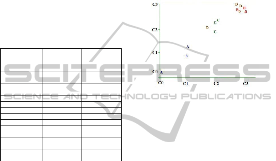
6.2.1 Unsupervised Learning – k-Means
Clustering
With reference to Figure 5, we can see the graphical
representation generated by Weka of the result of
running fold 1 of the data through the k-Means
clustering algorithm, with the number of clusters set
to four.
Figure 5: Plot of simple k-Means clustering. X:cluster
(nominal) Vs Y:cluster (nominal) with overlay of Class
variable (nominal).
Figure 5 illustrates the difficulty and ambiguity of
the instances defined in the training data set.
Tendency „A‟ (Phenomenon, continuous increase
decrease) is the most distinguishable although two
clusters C0 and C1 have been defined for it.
Tendency „C‟ (surge of interest) has been well
grouped as cluster C2. Tendencies „B‟ (specific
bursts) and „D‟ (periodic variation) are grouped
together as cluster C3, except for one instance of
tendency „D‟, which was grouped in cluster C2. In
the light of the clustering results, one future line of
work would be to try fuzzy clustering (e.g. fuzzy c-
Means) in which an instance may belong to more
than one cluster at the same time, with different
grades of membership.
6.2.2 Supervised Learners
In the following we show overall results for all
learners and for each tendency (Table 3); results for
each learner for each tendency (Table 4); and results
for each query term and each learner (Table 5).
With reference to the precision and recall, we
note that „precision‟ is related to the „false positive
rate‟ and that „recall‟ is related to the „true positive
rate‟. That is, „false positive‟ indicates the number of
instances of other classes assigned to the reference
class, and „true positive‟ indicates the number of
instances of the reference class which are correctly
assigned. In Table 3 we observe the overall
COLLECTIVE BEHAVIOUR IN INTERNET - Tendency Analysis of the Frequency of User Web Queries
173

precisions, and highlighted in grey we see that
tendencies A and D have given the best overall test
precisions. The lowest precision was given by
tendency B, as expected. We note that for tendency
types B and D the recall is superior to the precision,
whereas for tendencies A and C, precision and recall
are the same.
Table 3: Average train and test precision and recall % of
three learners for classifying each reference tendency.
Reference
Tendency
Train*
Test*
Pr.†
Re.‡
Pr.
Re.
A
100.00
93.40
100.00
100.00
B
48.87
48.87
43.33
60.00
C
100.00
84.60
66.67
66.67
D
67.22
85.80
66.04
86.18
Avg.*
79.02
78.17
69.01
78.21
†Pr.=Precision; ‡Re.=Recall; *Arithmetic mean per
tendency, of 5x2 fold cross-validation.
As was expected, tendencies A (steady increase) and
D (periodic variation) were the easiest to identify
and classify, with test precisions of 100% and
69.01%, respectively. Tendency B (specific bursts)
was more difficult to classify because of the ad-hoc
nature of the features and the presence of noise,
especially in the first part of the time period.
Tendency C (surge of interest) had a precision and
recall of 66.7%, and should have performed better,
although some noise and an ambiguous instance
(“michael jackson”) brought down the average.
With reference to Table 4, we observe the
precision and recall results for each tendency, and
for each supervised learning method. In grey we
have highlighted the relatively good results of RBF
for tendency B, the results of IBk for tendency C and
the results of SMO for tendency D. The best overall
precision (77.5) and recall (85.0) was given by IBk.
This coincides with other studies in which IBk has
proved robust in bench-markings with noisy datasets
(Nettleton, 2010).
Table 4: Average test precision of each learner for
classifying each reference tendency.
Reference
Tendency
RBF*
SMO*
IBk*
Pr. †
Re.
‡
Pr.
Re.
Pr.
Re.
A
100
100
100
100
100
100
B
60.0
100
20.0
20.0
50.0
60.0
C
40.0
40.0
60.0
60.0
100
100
D
80.0
80.0
60.0
100
60.0
80.0
Avg.*
70.0
80.0
60.0
70.0
77.5
85.0
†Pr.=Precision; ‡Re.=Recall; *Arithmetic mean per
tendency, of 5x2 fold cross-validation.
Table 5: Test Accuracy of three learners for classifying
tendencies of individual query terms.
Query
Term /Ref.
Tendency
RBF*
SMO*
IBk*
Pr.
†
Re.
‡
Pr.
Re.
Pr.
Re.
wiki (A)
1
1
1
1
1
1
yahoo(A)
1
1
1
1
1
1
google(A+B.1)
1
1
1
1
1
1
linux(A)
1
1
1
1
1
1
renault clio (B+D)
.5
1
1
1
.5
1
seat ibiza (B+D)
1
1
0
0
0
0
windows (B+D,A)
.5
1
0
0
0
0
electric car (B)
.5
1
0
0
1
1
ratzinger (C)
0
0
1
1
1
1
haiti (C)
1
1
1
1
1
1
tsunami (C)
1
1
1
1
1
1
michael jackson
(C)
0
0
0
0
1
1
xbox (D+B)
1
1
.5
1
1
1
ipod (D+B)
1
1
.5
1
.5
1
dvd (D+A)
0
0
.5
1
.5
1
mp3 (D+A)
0
0
1
1
0
0
imagenio (D+B)
1
1
.5
1
1
1
†Pr.=Precision; ‡Re.=Recall; *1, .5 and 0 refer to the
results for individual instances.
Table 5 is a disaggregated version of Table 4, in
which we can see the precision and recall results for
each learner, and for each individual query. We have
been able to obtain this information because of the
way we have designed the train and test folds, as
explained in Section 6.1 (Experimental Setup) of the
paper. The values represent individual
classifications: 1 is a correct classification, 0 is an
incorrect classification and 0.5 means that there was
a correct classification but there was also a false
positive or negative from another class.
We observe that the most difficult query term to
classify was “windows”, followed by “seat ibiza”,
“michael jackson” and “mp3”. Observation of the
plots of the trends of these queries shows that each
has some ambiguity, noise, ad-hoc nature or
deviation from the assigned tendency class. On the
other hand, the easiest to classify were all queries of
tendency A and “haiti” and “tsunami” of tendency
C. We can see that the RBF learner gave better
results than the other learners for the tendency B
queries “seat ibiza” and “windows”.
7 CONCLUSIONS
In this paper we have looked at some of the
background to collective behaviour theory, and we
have seen some practical examples from Google
Trends, showing the changing frequencies of user
KDIR 2010 - International Conference on Knowledge Discovery and Information Retrieval
174

internet search keywords over time. We have
defined a hypothetical classification of four major
trends types. Then we have applied three supervised
and one non-supervised learning techniques to
classify the example query trends into the
hypothetical categories. We conclude that it is
relatively easy to classify the given trends when they
are “pure”, although the precision suffers when the
example to be classified contains a mixture of
several trends, has noise, or are ad-hoc. This is a
common situation with real data. We have shown
that the IBk learning technique gives the best overall
results for precision (77.5%) and recall (85%) for
this classification task. Tendency types A
(phenomenon) and D (periodic variation) have given
the best classification results with (pr.=100%,
re.=100%) and (pr.=66,04%, re.=86,14%),
respectively.
There are many companies that try to influence
opinion about their products in Internet, by creating
and publishing contents. But even though the Web
2.0 has increased the number of content authors in
the web, their number is, and will to continue to be
smaller than the number of people who formulate
queries (content searchers). Also, the information
obtained from Internet search is cleaner, more
transparent and more difficult for competitors to
manipulate. With this paper we make a first study of
the evolution of user queries over time and the kind
of information that can be extracted from it. In
future work we expect to adjust mathematical
models on this data in order to be able to measure
the impact over time of a marketing campaign.
REFERENCES
Aizen, J., Huttenlocher, D., Kleinberg, J., Novak, A.
(2003). Traffic-Based Feedback on the Web.
Department of Computer Science, Cornell University.
Proceedings of the National Academy of Sciences.
Baeza-Yates, R., Hurtado, C., Mendoza, M. and Dupret G.
(2005). Modeling user search behavior. In Proceedings
of the Third Latin American Web Congress 2005, p.
242 – 251. Buenos Aires, Argentina, Oct. 2005.
Cacheda, F., and Viña, Á. (2001). Experiences retrieving
information in the world wide web. In Proceedings of
the 6th IEEE Symposium on Computers and
Communications, pp. 72-79. Hammamet, Tunisia.
July.
Cho, J. and Roy, S. (2004). Impact of Search Engines on
Page Popularity. In Proceedings of the Thirteenth
International World Wide Web Conference, New
York, USA, Pages: 20 – 29.
Choi, H., Varian, H (2009). Predicting Initial Claims for
Unemployment Benefits. Google Inc. -
research.google.com
Choi, H., Varian, H. (2010). Predicting the Present with
Google Trends. Google Inc., Draft -
www.googleresearch.blogspot.com
Google Trends. (2010). Google Inc.
www.google.com/trends
Hall, M., Eibe F., Holmes, G., Pfahringer, B., Reutemann,
P., Witten, I. (2009). The WEKA Data Mining
Software: An Update; SIGKDD Explorations, Volume
11, Issue 1.
Klienberg, J. (2002). Bursty and Hierarchical Structure in
Streams. Proceedings of the 8th ACM SIGKDD
International Conference on Knowledge Discovery
and Data Mining.
Nettleton, D.F., Baeza-Yates, R. (2008). Web retrieval:
Techniques for the aggregation and selection of
queries and answers. International Journal of
Intelligent Systems, Vol. 23/12 p1223-1234.
Nettleton, D.F., Orriols-Puig, A., Fornells, A. (2010). A
Study of the Effect of Different Types of Noise on the
Precision of Supervised Learning Techniques.
Artificial Intelligence Review, Ed. Springer, Vol. 33,
Num. 4, p275-306.
Rabiner, L. R. (1989). A Tutorial on Hidden Markov
Models and Selected Applications in Speech
Recognition. Proc. of the IEEE, Vol.77, No.2, pp.257-
286.
Rech, Jörg. (2007). Discovering trends in software
engineering with google trends. ACM SIGSOFT
Software Eng. Notes, Vol. 32 , Issue 2, Pages 1 – 2.
Silvestri, F. (2004). High Performance Issues in Web
Search Engines: Algorithms and Techniques. Ph. D.
Thesis TD 5/04. Universita degli studi di Pisa,
Dipartimento di Informatica, May 2004,
http://hpc.isti.cnr.it/~silvestr
Yu, S., Zhou, Z.H., Steinbach, M., Hand, D.J. &
Steinberg, D. (2007). Top 10 algorithms in data
mining. Knowledge and Inf. Systems, 14(1):1–37.
COLLECTIVE BEHAVIOUR IN INTERNET - Tendency Analysis of the Frequency of User Web Queries
175
