
EVOLUTIONARY ALGORITHMS FOR SOLVING QUASI
GEOMETRIC PROGRAMMING PROBLEMS
R. Toscano and P. Lyonnet
Universit´e de Lyon, Laboratoire de Tribologie et de Dynamique des Syst`emes, CNRS UMR5513 ECL/ENISE
58 rue Jean Parot 42023 Saint-Etienne cedex 2, France
Keywords:
Geometric Programming (GP), Quasi Geometric Programming (QGP), Evolutionary Algorithm (EA), Interior
point method.
Abstract:
In this paper we introduce an extension of standard geometric programming (GP) problems which we call
quasi geometric programming (QGP) problems. The consideration of this particular kind of nonlinear and
possibly non smooth optimization problem is motivated by the fact that many engineering problems can be
formulated as a QGP. However, solving a QGP remains a difficult task due to its intrinsic non-convex nature.
This is why we investigate the possibility of using evolutionary algorithms (EA) for solving a QGP problem.
The main idea developed in this paper is to combine evolutionary algorithms with interior point method for
efficiently solving QGP problems. An interesting feature of the proposed approach is that it does not need
to develop specific program solver and works well with any existing EA and available solver able to solve
conventional GP. Some considerations on the robustness issue are also presented. Numerical experiments are
used to validate the proposed method.
1 INTRODUCTION
Geometric programming (GP) has proved to be a very
efficient tool for solving various kinds of engineering
problems. This efficiency comes from the fact that
geometric programs can be transformed to convexop-
timization problems for which powerful global opti-
mization methods have been developed. As a result,
globally optimal solution can be computed with great
efficiency, even for problems with hundreds of vari-
ables and thousands of constraints, using recently de-
veloped interior-point algorithms. A detailed tutorial
of GP and comprehensive survey of its recent appli-
cations to various engineering problems can be found
in (Boyd et al., 2007).
In this paper we introduce an important extension
of GP which we call quasi geometric programming
(QGP) problems. The motivation of introducing this
particular kind of nonlinear program comes from the
fact that a lot of engineering problems can be formu-
lated as a QGP. Thus, solving a given QGP appears of
great practical importance.
A major difficulty is that QGP is a nonlinear
non-convex and possibly non smooth optimization
problem. This is a major source of computational
intractability and conservatism (Rockafellar, 1993),
(Boyd and Vandenberghe, 2004). Indeed, unlike GP
problems, QGP problems remain non-convex in both
their primal and dual forms and there is no transfor-
mation able to convexify them. Consequently, only a
locally optimal solution of a QGP can be computed
efficiently
1
.
On the other hand, evolutionary algorithms (EAs)
have demonstrated a strong ability to deal with non-
convex optimization problems. Indeed, EAs maintain
several solutions simultaneously, which provide a sig-
nificantly better foundation for escaping from local
optima. In addition, solutions are not necessarily cre-
ated as neighbors of existing solutions and thus, this
increases the probability of finding the global opti-
mum. Over the years, a lot of algorithms have been
suggested, however the basic principles remain the
same and a good overview can be found in (Back
and Schwefel., 1993), (Michalewicz and Schoenauer.,
1996).
The main idea developed in this paper is to asso-
ciate the interior point method, able to solve very effi-
ciently a GP problem, with the ability of evolutionary
1
It is possible to compute the globally optimal solution
of a QGP, but this can require prohibitive computation, even
for relatively small problems.
163
Toscano R. and Lyonnet P..
EVOLUTIONARY ALGORITHMS FOR SOLVING QUASI GEOMETRIC PROGRAMMING PROBLEMS.
DOI: 10.5220/0003071901630169
In Proceedings of the International Conference on Evolutionary Computation (ICEC-2010), pages 163-169
ISBN: 978-989-8425-31-7
Copyright
c
2010 SCITEPRESS (Science and Technology Publications, Lda.)

algorithms of dealing with non-convex optimization
problems. This is possible because a QGP becomes
a GP when some variables are kept constant. The in-
teresting thing is that the proposed approach does not
need to develop specific program solver and works
well with any existing evolutionary algorithm (for
instance a standard genetic algorithm) and available
solver able to solve conventional geometric programs
(for instance cvx (Grant and Boyd, 2010)). From a
practical point of view this is very interesting because
the engineers often have not so much time to develop
specific algorithm for solving particular problems.
The rest of this paper is organized as follows. In
section 2, we provide a short introduction to GP. Sec-
tion 3 is the main part of this paper. It introduces the
notion of quasi geometric programming problems as
well as their resolutions using available EAs and GP
solvers. In many practical problems some parameters
are not precisely known, this aspect is discussed in
section 4 which is devoted to the robustness issue. In
section 5 some optimization problems are considered
to illustrate the validity of the proposed method for
solving a QGP problem. We give concluding remarks
in section 6.
2 GEOMETRIC PROGRAMMING
GP is a special type of nonlinear, non-convex optimi-
sation problems. An useful property of GP is that it
can be turned into a convexoptimization problem and
thus a local optimum is also a global one, which can
be computed very efficiently. Since QGP is based on
the resolution of GP, this section gives a short presen-
tation of GP both in standard and convex form.
2.1 Standard Formulation
Monomials are the basic elements for formulating a
geometric programming problem. A monomial is a
function f : R
n
++
→ R defined by
2
:
f(x) = cx
a
1
1
x
a
2
2
···x
a
n
n
(1)
where x
1
,···x
n
are n positive variables, c is a positive
multiplicative constant and the exponentials a
i
, i =
1,··· , n are real numbers. We will denote by x the
vector (x
1
,··· ,x
n
). A sum of monomial is called a
posynomial:
f(x) =
K
∑
k=1
c
k
x
a
1
k
1
x
a
2
k
2
···x
a
n
k
n
(2)
2
In our notations, R
++
represents the set of positive real
numbers.
Minimizing a posynomial subject to posynomial up-
per bound inequality constraints and monomial equal-
ity constraints is called GP in standard form:
minimize f
0
(x)
subject to f
i
(x) 6 1, i = 1,··· , m
g
i
(x) = 1, i = 1,··· , p
(3)
where f
i
, i = 0, · · · , m, are posynomials and g
i
, i =
1,··· , p, are monomials.
2.2 Convex Formulation
GP in standard form is not a convex optimisation
problem
3
, but it can be transformed to a convex prob-
lem by an appropriate change of variables and a log
transformation of the objective and constraint func-
tions. Indeed, if we introduce the change of variables
y
i
= logx
i
(and so x
i
= e
y
i
), the posynomial function
(2) becomes:
f(y) =
K
∑
k=1
c
k
exp
n
∑
i=1
a
i
k
y
i
!
=
K
∑
k=1
exp(a
T
k
y+ b
k
)
(4)
where b
k
= logc
k
, taking the log we obtain
¯
f(y) =
log
∑
K
k=1
exp(a
T
k
y+ b
k
)
, which is a convex function
of the new variable y. Applying this change of vari-
able and the log transformation to the problem (3)
gives the following equivalent optimization problem:
minimize
¯
f
0
(y) = log
∑
K
0
k=1
exp(a
T
0k
y+ b
0k
)
subject to
¯
f
i
(y) = log
∑
K
i
k=1
exp(a
T
ik
y+ b
ik
)
6 0
¯g
j
(y) = a
T
j
y+ b
j
= 0
(5)
where i = 1, · · · , m and j = 1, · · · , p. Since the func-
tions
¯
f
i
are convex, and ¯g
j
are affine, this problem
is a convex optimization problem, called geometric
program in convex form. However, in some practical
situations, it is not possible to formulate the problem
in standard geometric form, the problem is then not
convex. In this case the problem is generally diffi-
cult to solve even approximately. In these situations,
it seems very useful to introduce simple approaches
able to give if not the optimum, at least a good near-
optimum. In this spirit, we are now ready to introduce
the concept of quasi geometric programming.
3
A convex optimization problem consists in minimizing
a convex function subject to convex inequality constraints
and linear equality constraints.
ICEC 2010 - International Conference on Evolutionary Computation
164

3 QUASI GEOMETRIC
PROGRAMMING (QGP)
Consider the nonlinear program defined by
minimize f
0
(z)
subject to f
i
(z) 6 0, i = 1,··· ,m
g
j
(z) = 0, j = 1,··· , p
(6)
where the vector z ∈ R
n
++
include all the optimiza-
tion variables, f
0
: R
n
++
→ R is the objective func-
tion or cost function, f
i
: R
n
++
→ R are the inequality
constraint functions and g
j
: R
n
++
→ R are the equal-
ity constraint functions. This nonlinear optimization
problem is called a quasi geometric programming
problem if it can be formulated into the following
form:
minimize ϕ
0
(x,ξ) − ϕ
′
0
(ξ)
subject to ϕ
i
(x,ξ) 6 Q
i
(ξ), i = 1, · · · , m
h
j
(x,ξ) = Q
′
j
(ξ), j = 1,··· , p
(7)
where x ∈ R
n
x
++
and ξ ∈ R
n
ξ
++
with n
x
+ n
ξ
= n, are
sub-vector of the optimization variable z ∈ R
n
++
. The
functions ϕ
i
(x,ξ), i = 0, · · · , m are posynomials and
h
j
(x,ξ), j = 1,··· , p are monomials. The only par-
ticular assumption made about the functions ϕ
′
0
(ξ),
Q
i
(ξ) and Q
′
j
(ξ), is that they are positives. Except
for their positivity, no other particular assumption is
made; these functions can be even non-smooth.
The QGP (7) can be reformulated as follows:
maximize λ
subject to λ 6 −ϕ
0
(x,ξ) + ϕ
′
0
(ξ)
ϕ
i
(x,ξ) 6 Q
i
(ξ), i = 1, · · · ,m
h
j
(x,ξ) = Q
′
j
(ξ), j = 1,··· , p
(8)
where λ ∈ R
++
is an additional decision variable. It
is important to insist on the fact that the problem (7),
or equivalently (8), cannot be converted into a GP in
the standard form (3) and thus the problem is not con-
vex. As a consequence, no approach exists for finding
quickly even a sub optimal solution by using available
GP solvers. Although specific algorithms can be de-
signed to find out a sub optimal solution to problem
(8), we think that it could be very interesting solving
these problems by using available EA and standard
GP solvers. Indeed, this could be interesting for at
least two reasons. Firstly the ability of solving prob-
lem (8) using available GP solvers allows time sav-
ing; the development of a specific algorithm is always
a long process and in an industrial context of great
concurrency there is often no time to do that. Sec-
ondly, the available GP solvers like for instance cvx
are very easy to use and, which is most important, are
very very efficient. Problems involving tens of vari-
ables and hundreds of constraints can be solved on
a small current workstation in less than one second.
All these reasons justify the approach presented here
after. Indeed, this method does not require the devel-
opment of particular algorithms and is based on the
use of available EA and GP solvers.
The QGP (8) is not at all easy to solve when ϕ
′
0
(ξ),
Q
i
(ξ) and Q
′
j
(ξ) have no particular form. In this case
indeed, the problem is intrinsically non-convex, and
thus, in general, there is no obvious transformation
allowing to solve (8) via the resolution of a sequence
of standard GP. To solve this kind of problem, we can
see the QGP (7), or equivalently (8), as a function of
ξ, denoted J(ξ), that we want to maximize:
maximize J(ξ)
subject to ξ 6 ξ 6
¯
ξ
(9)
where ξ and
¯
ξ are simple bound constraints on the
decision variable ξ, and the function J(ξ) is defined
as follows:
J(ξ) = max
x,λ
λ
subject to
λ+ ϕ
0
(x,ξ)
ϕ
′
0
(ξ)
6 1
ϕ
i
(x,ξ)
Q
i
(ξ)
6 1, i = 1,··· ,m
h
j
(x,ξ)
Q
′
j
(ξ)
= 1, j = 1,··· , p
(10)
Problem (9) is a non-convex unconstrained opti-
mization problem
4
and can be solved using evolution-
ary algorithms
5
like, for instance, a standard genetic
algorithm (GA). The code associated to this kind of
algorithms is easily available and thus don’t need to
be programmed.
When ξ is kept constant, problem (10) is a stan-
dard GP which can be solved very efficiently using
available GP solvers.
This suggests that we can solve the QGP problem
(8) with a two levels procedure. At the first level, the
chosen EA (eg. the standard GA) is used to select val-
ues of ξ within the bounds. For each value of ξ, the
standard GP (10) is solved using available solvers. As
we can see, (10) is our fitness function which is eval-
uated by solving a standard GP problem. This proce-
dure is continued until some stopping rule is satisfied.
The suggested procedure is formalized more precisely
in the following algorithm.
4
We have only simple bound constraints on the decision
variable ξ.
5
Note that EAs does not require the knowledge of the
derivatives of the objective function. Thus, smoothness is
not required.
EVOLUTIONARY ALGORITHMS FOR SOLVING QUASI GEOMETRIC PROGRAMMING PROBLEMS
165

Algorithm for Solving a QGP Problem (EA-QGP)
1. Set k := 0,
best
:= −
inf
, ξ
opt
:= −1 and x
opt
:=
−1 or other infeasible values.
2. Using an EA, generate a population P(k) =
n
ξ
(k)
i
o
i=I
i=1
, such that ξ 6 ξ
(k)
i
6
¯
ξ, for all individ-
uals i; I is the size of the population.
3. For each individual ξ
(k)
i
solve the standard GP
problem (10) w.r.t λ and x. This gives, w.r.t ξ
(k)
i
,
the optimal solution denoted λ
(k)
i
and x
(k)
i
. This
step represents the evaluation of the population
P(k). If problem (10) is not feasible, then set
J(ξ
(k)
) := −
inf
else set J(ξ
(k)
) := λ
(k)
.
4. If J(ξ
(k)
b
) >
best
, then set:
best
:= J(ξ
(k)
b
),
ξ
opt
:= ξ
(k)
b
and x
opt
:= x
(k)
b
, where ξ
(k)
b
represents
the best individual of the population P(k) and x
(k)
b
the solution to the corresponding GP problem.
5. If the termination condition is satisfied, go to step
7 (the termination condition can be, for instance,
a defined number of iterations).
6. From the results obtained step 3, generate a new
population P(k) where k := k + 1 (this is done by
using the usual operators of EA, i.e. selection,
crossover and mutation operators), go to step 3.
7. The optimal solution is given by (x
opt
,ξ
opt
), stop.
In this algorithm,
inf
represents the IEEE arith-
metic representation for positive infinity, and
best
is
a variable containing the current best objective func-
tion. Note that the use of “ global optimization meth-
ods ” like, for instance GA, increases the probability
of finding a global optimum but this is not guaran-
teed, except perhaps if the search space of problem
(9) is explored very finely, but this cannot be done in
a reasonable time.
4 ROBUSTNESS ISSUE
Until now it was implicitly assumed that the parame-
ters (i.e. the problem data) which enter in the formu-
lation of a QGP problem are precisely known. How-
ever, in many practical applications some of these pa-
rameters are subject to uncertainties. It is then im-
portant to be able to calculate solutions that are in-
sensitive to parameters uncertainties; this leads to the
notion of optimal robust design. We say that the de-
sign is robust, if the various specifications (i.e. the
constraints) are satisfied for a set of values of the pa-
rameters uncertainties. In this section we show how
to use the methods presented above to developdesigns
that are robust with respect to some parameters uncer-
tainties.
Let θ = [θ
1
θ
2
··· θ
q
]
T
be the vector of uncertain
parameters. It is assumed that θ lie in a bounded set
Θ defined as follows:
Θ =
θ ∈ R
q
: θ θ
¯
θ
, (11)
where the notation denotes the componentwise in-
equality between two vectors: v w means v
i
6 w
i
for all i. The vectors θ = [θ
1
···θ
q
]
T
,
¯
θ = [
¯
θ
1
···
¯
θ
q
]
T
are the bounds of uncertainty of the parameters vec-
tor θ. Thus, the uncertain vector belong to the q-
dimensional hyperrectangle Θ also called the param-
eter box. In these conditions, the QGP problem (7),
or equivalently (8), must be expressed in term of func-
tions of (x,ξ), the design variables, and θ the vector of
uncertain parameters. The robust version of the quasi
geometric problem (8) is then written as follows:
maximize λ
subject to λ+ ϕ
0
(x,ξ,θ) 6 ϕ
′
0
(ξ,θ)
ϕ
i
(x,ξ,θ) 6 Q
i
(ξ,θ), i = 1,··· ,m
h
j
(x,ξ,θ) = Q
′
j
(ξ,θ), j = 1,··· , p
(12)
for all θ ∈ Θ. The functions ϕ
i
, i = 0,··· , m, are
posynomial functions of (x,ξ), for each value of θ,
and the functions h
j
, j = 1, · · · , p, are monomial func-
tions of (x,ξ), for each value of θ. The functions ϕ
′
0
,
Q
i
and Q
′
j
are only assumed to be positive for each θ.
We consider the resolution of the robust QGP
problem in the case of a finite set. Let Θ
N
=
{θ
(1)
, θ
(2)
,··· ,θ
(N)
} be a finite set of possible vec-
tor parameter values. This finite set can be imposed
by the problem itself or can be obtained by sampling
the continuous set Θ defined in (11). For instance, we
might sample each interval [θ
i
,
¯
θ
i
] with three values:
θ
i
,
θ
i
+
¯
θ
i
2
and
¯
θ
i
, and form every possible combination
of parameter values, this lead to N = 3
q
different vec-
tor parameters.
Whatever how the finite set is obtained, we have to
determine a solution (x, ξ) that satisfy the QGP prob-
lem for all possible vector parameters. To do so, we
have only to replicate the constraints for all possible
vector parameters. Thus, in the case of a finite set Θ
N
,
the robust QGP problem is formulated as follows:
maximize λ
subject to λ+ ϕ
0
(x,ξ,θ
(k)
) 6 ϕ
′
0
(ξ,θ
(k)
)
ϕ
i
(x,ξ,θ
(k)
) 6 Q
i
(ξ,θ
(k)
)
h
j
(x,ξ,θ
(k)
) = Q
′
j
(ξ,θ
(k)
)
(13)
where i = 1,··· ,m and j = 1,··· , p and k = 1,··· ,N.
As we can see, problem (13) can be solved as a stan-
ICEC 2010 - International Conference on Evolutionary Computation
166
dard QGP problem using the method presented in sec-
tion 3.
5 NUMERICAL EXAMPLES
In this section we illustrate the applicability of the
proposed method through three numerical examples.
In these examples, the EA-QGP has been imple-
mented using the GA toolbox (Chipperfield et al.,
1995) and the GP solver cvx (Grant and Boyd, 2010).
The following parameters were used: binary coded-
GA 16 bits, number of generations 30 (used as stop-
ping rule), population size 20, roulette wheel selec-
tion, one point crossover with probability of 0.7 and
a probability of mutation 0.07. The number of gener-
ations has been chosen deliberately small to avoid a
too long computation time. Indeed, the time cost for
a GP-solver call (in the three examples this time cost
is about 0.5s) is generally higher than the time cost of
the objective function. The price to pay is that the so-
lution thus found is not necessarily the best possible.
5.1 Example 1
This first example is borrowed from (Qu et al., 2007)
in which the problem was solved using a global op-
timization algorithm via lagrangian relaxation (GD-
CAB).
min. 0.5t
1
t
−1
2
− t
1
− 5t
−1
2
s. t. 0.01t
2
t
−1
3
+ 0.01t
2
+ 0.0005t
1
t
3
6 1
70 6 t
1
6 150, 1 6 t
2
6 30, 0.5 6 t
3
6 21
This problem can be rewritten as follows:
max. λ
s. t.
λ+ 0.5t
1
t
−1
2
t
1
+ 5t
−1
2
6 1
0.01t
2
t
−1
3
+ 0.01t
2
+ 0.0005t
1
t
3
6 1
70 6 t
1
6 150, 1 6 t
2
6 30, 0.5 6 t
3
6 21
which is QGP in (t
1
, t
2
). The method EA-QGP de-
scribed section 3, was applied to solve this optimiza-
tion problem and the solution found is presented in
Table 1. It can be seen that the solution found using
EA-QGP is very significantly better than that found
using the method described in (Qu et al., 2007).
Note also that the Number of iterations (in fact,
the number of GP-solver call) is small compared to
the number of iterations required by GDCAB. How-
ever, recall that the time cost of a GP-solver call is
generally higher than the computation time of the ob-
jective function.
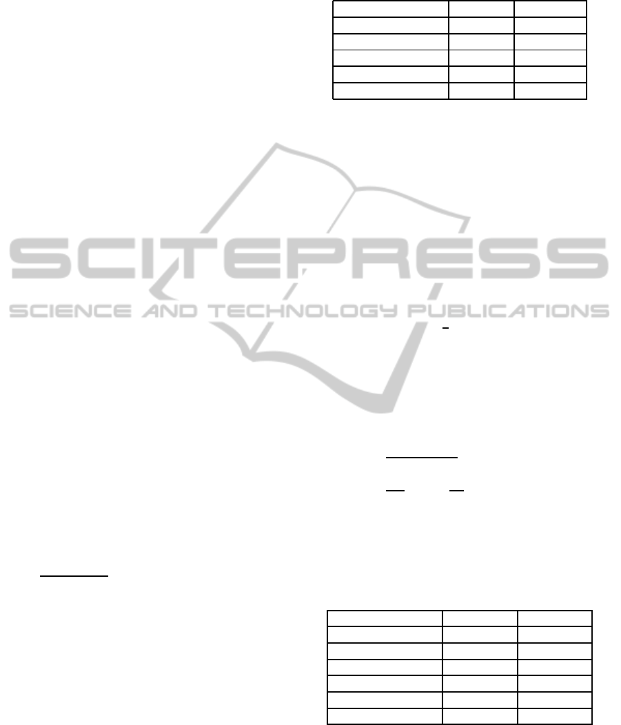
Table 1: Comparison of the solution found by EA-QGP and
GDCAB see (Qu et al., 2007)
GDCAB EA-QGP
t
1
88.6274 149.9999
t
2
7.9621 18.9558
t
3
1.3215 1.6973
objective function -83.6898 -146.3064
NbIter 1754 600
5.2 Example 2
This second example is borrowed from (He and
Wang., 2007) in which the problem was solved us-
ing a co-evolutionary particle swarm optimization
(CPSO). In this problem, the objective is to minimize
the total cost including the cost of the material, form-
ing and welding of a cylindrical vessel.
min. 0.6224x
1
x
3
x
4
+ 1.7778x
2
x
2
3
+3.1661x
2
1
x4+ 19.84x
2
1
x
3
s. t. −x
1
+ 0.0193x
3
6 0
−x
2
+ 0.009543x
3
6 0
−πx
2
3
x
4
−
4
3
πx
3
3
+ 1296000 6 0
1 6 x
1
, x
2
6 99, 10 6 x
3
, x
4
6 200
This problem can be reformulated as follows:
min. 0.6224x
1
x
3
x
4
+ 1.7778x
2
x
2
3
+3.1661x
2
1
x4+ 19.84x
2
1
x
3
s. t. −0.0193x
3
/x
1
6 1
0.009543x
3
/x
2
6 1
1296000
πx
3
3
(z+ 4/3)
6 1
x
4
x
3
z
= 1,
1
20
6 z 6 20
1 6 x
1
, x
2
6 99, 10 6 x
3
, x
4
6 200
which is QGP in z. The solution found using the EA-
QGP method is presented in Table 2.
Table 2: Comparison of the solution found by EA-QGP and
CPS0 see (He and Wang., 2007)
CPSO EA-QGP
x
1
0.8125 0.7782
x
2
0.4375 0.3846
x
3
42.0913 40.3197
x
4
176.7465 199.9993
objective function 6061.0777 5885.3336
NbFuncEval 32500 600
From Table 2, it can be seen that the solution
found using EA-QGP is significantly better than that
found using the method described in (He and Wang.,
2007). Regarding the number of function evaluations
(NbFuncEval) the same remark as in example 1 ap-
plies.
EVOLUTIONARY ALGORITHMS FOR SOLVING QUASI GEOMETRIC PROGRAMMING PROBLEMS
167
5.3 Example 3
This third and last example is borrowed from (Cagn-
ina et al., 2008) in which the problem was solved
using a constrained particle swarm optimizer (SiC-
PSO). This problem is related to the design of a speed
reducer. The objective is to minimize the weight of
the speed reducer subject to constraints on bending
stress of the gear teeth, surface stress, transverse de-
flections of the shafts and stresses in the shaft. The
corresponding optimization problem were formulated
as follows:
min. 0.7854x
1
x
2
2
(3.3333x
2
3
+ 14.9334x
3
− 43.0934)
−1.508x
1
(x
2
6
+ x
2
7
) + 7.4777(x
3
6
+ x
3
7
)
+0.7854(x
4
x
2
6
+ x
5
x
2
7
)
s. t.
27
x
1
x
2
2
x
3
6 1,
397.5
x
1
x
2
2
x
2
3
6 1
1.93x
3
4
x
2
x
3
x
4
6
6 1,
1.93x
3
5
x
2
x
3
x
4
7
6 1
1.0
110x
3
6
s
745.0x
4
x
2
x
3
2
+ 16.9 × 10
6
6 1
1.0
85x
3
7
s
745.0x
5
x
2
x
3
2
+ 157.5 × 10
6
6 1
x
2
x
3
40
6 1,
5x
2
x
1
6 1,
x
1
12x
2
6 1
1.5x
6
+ 1.9
x
4
6 1,
1.1x
7
+ 1.9
x
5
6 1
2.6 6 x
1
6 3.6, 0.7 6 x
2
6 0.8, 17 6 x
3
6 28
7.3 6 x
4
6 8.3, 7.8 6 x
5
6 8.3, 2.9 6 x
6
6 3.9
5.0 6 x
7
6 5.5
To apply the proposed approach, this problem can be
rewritten into the following form:
max. λ
s. t. λ+ ϕ
0
6 ϕ
′
0
27
x
1
x
2
2
x
3
6 1,
397.5
x
1
x
2
2
x
2
3
6 1
1.93x
3
4
x
2
x
3
x
4
6
6 1,
1.93x
3
5
x
2
x
3
x
4
7
6 1
1.0
110x
3
6
s
745.0x
4
x
2
x
3
2
+ 16.9 × 10
6
6 1
1.0
85x
3
7
s
745.0x
5
x
2
x
3
2
+ 157.5 × 10
6
6 1
x
2
x
3
40
6 1,
5x
2
x
1
6 1,
x
1
12x
2
6 1
1.5x
6
+ 1.9
x
4
6 1,
1.1x
7
+ 1.9
x
5
6 1
2.6 6 x
1
6 3.6, 0.7 6 x
2
6 0.8, 17 6 x
3
6 28
7.3 6 x
4
6 8.3, 7.8 6 x
5
6 8.3, 2.9 6 x
6
6 3.9
5.0 6 x
7
6 5.5
where ϕ
0
and ϕ
′
0
are defined as follows:
ϕ
0
= 0.7854x
1
x
2
2
x
3
(3.3333x
3
+ 14.9334)
+7.4777(x
3
6
+ x
3
7
) + 0.7854(x
4
x
2
6
+ x
5
x
2
7
)
ϕ
′
0
= 33.8456x
1
x
2
2
+ 1.508x
1
(x
2
6
+ x
2
7
)
Thus, this equivalent problem is QGP in
(x
1
,x
2
,x
6
,x
7
). The solution found using the
EA-QGP method is presented in Table 3. Note that
in spite of the square roots, the two equation are
still posynomials. From Table 3, it can be seen that
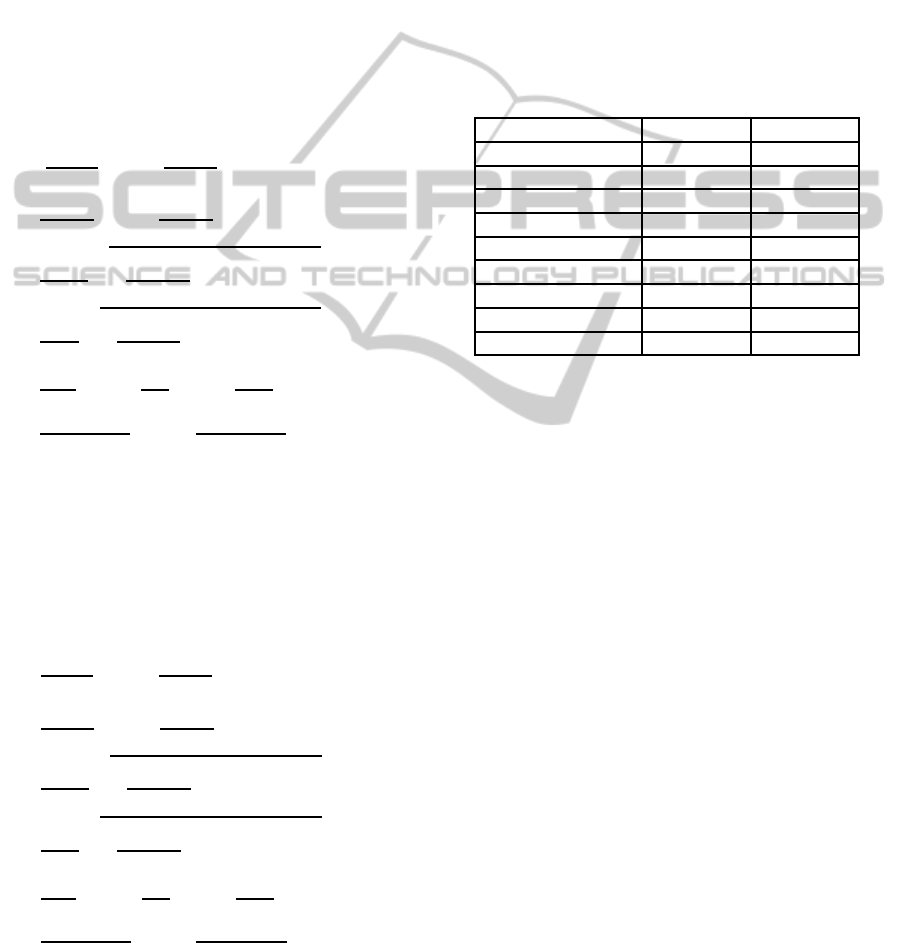
Table 3: Comparison of the solution found by EA-QGP and
SiC-PS0 see (Cagnina et al., 2008)
SiC-PSO EA-QGP
x
1
3.5000 3.5531
x
2
0.7000 0.6684
x
3
17 17
x
4
7.3000 7.3000
x
5
7.8000 7.8000
x
6
3.3502 3.3509
x
7
5.2867 5.2868
objective function 2996.3481 2876.4999
NbFuncEval 24000 600
the solution found using EA-QGP is better than that
found using the method described in (Cagnina et al.,
2008). Here also, regarding the number of function
evaluations (NbFuncEval) the same remark as in
example 1 applies.
6 CONCLUSIONS
In this paper, an important extension of standard ge-
ometric programming (GP), called quasi geometric
programming (QGP) problems, was introduced. The
consideration of this kind of problems is motivated
by the fact that many engineering problems can be
formulated as a QGP. Thus the problem of solving
a given QGP appears of great practical importance.
However, the resolution of a QGP is difficult due to
its non-convex nature. The main contribution of this
paper was to show that a given QGP can be efficiently
solved by combining evolutionary algorithms (EA)
and interior point methods. In addition, the proposed
approach does not need to develop specific program
solver and works well with any existing EA and avail-
able solver able to solve conventional GP. This fea-
ture is important for time saving reasons. Numerical
applications have shown that the results obtained by
applying the proposed method are better than those
obtained via any other approaches. This is not so
ICEC 2010 - International Conference on Evolutionary Computation
168

surprising since we don’t use EA in a blind man-
ner. On the contrary, the proposed approach takes
into account the particular structure of the problem
to be solved. Indeed, QGP becomes a standard GP
when some variables are kept constant. This impor-
tant property has suggested a resolution method in-
cluding two levels. At the first level, the ability of
EA to to deal with non-convex problems is exploited
and at the second level, the ability of interior point
method for solving a standard GP is used. This two
levels structure makes the resolution of a QGP effi-
cient and easy to do by using available EA and stan-
dard GP solver. However, the main drawback of the
proposed approach is that we have to choose a small
number of generations to prevent a too long compu-
tation time. This is a serious limitation since the so-
lution thus found is not necessarily the best possible.
From this point of view, the proposed approach needs
to be improved. One possible way is to generate the
initial population from a good approximate solution.
This approximate solution can be found using EA in
a usual way. In this case, the EA-QGP plays the role
of a refinement procedure.
REFERENCES
Back, T. and Schwefel., H. P. (1993). An overview of evo-
lutionary algorithms for parameter optimization. Evo-
lutionary Computation, 1(1):1–23.
Boyd, S., Kim, S.-J., Vandenberghe, L., and Hassibi., A.
(2007). A tutorial on geometric programming. Opti-
mization and Engineering, 8(1):67–127.
Boyd, S. and Vandenberghe, L. (2004). Convex optimiza-
tion. Cambridge University Press.
Cagnina, L. C., Esquivel, S. C., and Coello., C. A. C.
(2008). Solving engineering optimization problems
with the simple constrained particle swarm optimizer.
Informatica, 32(3):319–326.
Chipperfield, A., Fleming, P., Pohlheim, H., and Fonseca,
C. (1995). Genetic Algorithm TOOLBOXFor Use with
MATLAB.
Grant, M. and Boyd, S. (2010). CVX: Matlab Software
for Disciplined Convex Programming, version 1.21.
http://cvxr.com/cvx.
He, Q. and Wang., L. (2007). An effective co-evolutionary
particle swarm optimization for constrained engineer-
ing design problems. Engineering Application of Ar-
tificial Intelligence, 20(1):89–99.
Michalewicz, Z. and Schoenauer., M. (1996). Evolution-
ary algorithms for constrained parameter optimization
problems. Evolutionary Computation, 4(1):1–32.
Qu, S. J., Zhang, K. C., and Ji., Y. (2007). A new global
optimization algorithm for signomial geometric pro-
gramming via lagrangian relaxation. Applied Mathe-
matics and Computation, 184(2):886–894.
Rockafellar, R. T. (1993). Lagrange multipliers and opti-
mality. SIAM Review, 35:183–238.
EVOLUTIONARY ALGORITHMS FOR SOLVING QUASI GEOMETRIC PROGRAMMING PROBLEMS
169
