NEURAL NETWORK BASED HAMMERSTEIN

SYSTEM IDENTIFICATION

USING PARTICLE SWARM SUBSPACE ALGORITHM

S. Z. Rizvi and H. N. Al-Duwaish

Department of Electrical Engineering, King Fahd Univ. of Petroleum & Minerals, Dhahran, Saudi Arabia

Keywords:

Particle swarm optimization, Neural network training, Subspace identiﬁcation, Static nonlinearity, Dynamic

linearity, Radial basis function (RBF) neural networks.

Abstract:

This paper presents a new method for modeling of Hammerstein systems. The developed identiﬁcation method

uses state-space model in cascade with radial basis function (RBF) neural network. A recursive algorithm

is developed for estimating neural network synaptic weights and parameters of the state-space model. No

assumption on the structure of nonlinearity is made. The proposed algorithm works under the weak assumption

of richness of inputs. The problem of modeling is solved as an optimization problem and Particle Swarm

Optimization (PSO) is used for neural network training. Performance of the algorithm is evaluated in the

presence of noisy data and Monte-Carlo simulations are performed to ensure reliability and repeatability of

the identiﬁcation technique.

1 INTRODUCTION

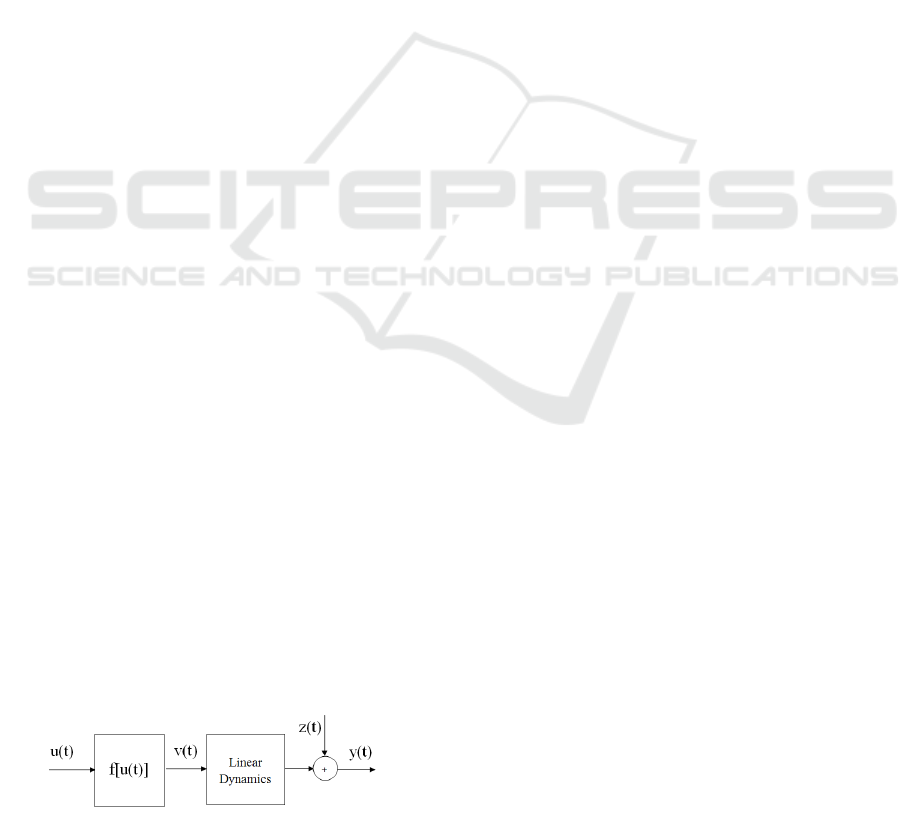
The Hammerstein Model belongs to the family of

block oriented models and is made up of a memory-

less nonlinear part followed by a linear dynamic part

as shown in Figure 1. It has been known to effectively

represent and approximate several nonlinear dynamic

industrial processes, for example pH neutralization

process (Fruzzetti, K. P., Palazoglu A., McDonald,

K. A., 1997), heat exchanger (Eskinat, E., Johnson,

S. H., Luyben, W. L., 1991), nonlinear ﬁlters (Had-

dad, A. H., Thomas, J. B., 1968), and water heater

(Abonyi, I., Nagy, L., Szeifert, E., 2000).

Figure 1: Block diagram of a Hammerstein model.

A lot of research has been carried out on identi-

ﬁcation of Hammerstein models. Hammerstein Sys-

tems can be modeled by employing either nonpara-

metric or parametric models. Nonparametric mod-

els represent the system in terms of curves result-

ing from expansion of series such as the Volterra se-

ries or kernel regression. Parametric representations

are more compact having fewer parameters. Notable

parametric identiﬁcation techniques can be found in

(Narendra, K. S., Gallman, P., 1966), (Billings, S.,

1980), (Al-Duwaish, H., 2001), (V¨or¨os, J., 2002),

(Wenxiao, Z., 2007) and in references therein. Non-

parametric identiﬁcation techniques can be found in

several papers including, but not limited to those of

(Greblicki, W., 1989), (Al-Duwaish, H., Nazmulka-

rim, M., Chandrasekar, V., 1997), (Zhao, W., Chen,

H., 2006).

Recently, subspace identiﬁcation has emerged as

a well known method for identiﬁcation of linear

systems. It is computationally less complicated as

compared to conventional prediction error methods

(PEM), does not require initial estimate of a canon-

ical model like PEM and, is easily extendable to sys-

tems having multiple inputs and outputs (Katayama,

T., 2005). However, its use is restricted mostly to lin-

ear systems. To make use of this, attempts have been

made to extend subspace linear identiﬁcation to non-

linear systems such as Wiener and Hammerstein sys-

tems including use of static nonlinearity in the feed-

back path (Luo, D., Leonessa, A., 2002), assuming

known nonlinearity structures (Verhaegen, M., West-

wick, D., 1996), and using least squares support vec-

tor machines (Goethals, I., Pelckmans, K., Suykens,

J. A. K., Moor, B. D., 2005).

In this paper, a new subspace based method is pro-

182

Z. Rizvi S. and N. Al-Duwaish H..

NEURAL NETWORK BASED HAMMERSTEIN SYSTEM IDENTIFICATION USING PARTICLE SWARM SUBSPACE ALGORITHM.

DOI: 10.5220/0003072401820189

In Proceedings of the International Conference on Fuzzy Computation and 2nd International Conference on Neural Computation (ICNC-2010), pages

182-189

ISBN: 978-989-8425-32-4

 2010 SCITEPRESS (Science and Technology Publications, Lda.)

posed for Hammerstein model identiﬁcation, which

uses radial basis function (RBF) network in cascade

with a state-space model. A recursive algorithm is

developed for parameter estimation of the two sub-

systems.

The paper is arranged as follows. Section 2 looks

at the model structure proposed in this work. Section

3 takes a detailed look at the proposed identiﬁcation

scheme. Section 4 describes the proposed algorithm

in detail and section 5 includes numerical examples,

their results, and analysis.

Throughout this paper, the following convention

is used for notations. Lower case variables represent

scalars. Lower case bold variables represent vectors.

Upper case bold letters denote matrices. The only ex-

ception to this convention is the choice of variable for

the cost function, where a more coventional J is used

to deﬁne the cost function.

2 PROPOSED MODEL

STRUCTURE

The proposed model structure in this work uses state-

space model to estimate the linear dynamic part. The

memoryless nonlinear part is modeled using an RBF

network. An RBF network is an effective type of neu-

ral network that has proved useful in applications like

function approximation and pattern recognition. A

typical three layer RBF network is shown in Figure

2. The input layer connects the network to its en-

vironment. The second layer, known as the hidden

layer, performs a ﬁxed nonlinear transformation us-

ing basis functions. The output layer linearly weighs

the response of the network to the output (Haykin,

S., 1999). The external inputs to the system u(t) are

fed to the RBF network, which generates the outputs

v(t). Considering an RBF network having q number

of neurons in the hidden layer, the basis vector is

φ(t) = [φku(t) − c

k···φku(t) − c

k],

where c

is the chosen center for the i

neuron, k.k

denotes norm that is usually Euclidean, and φ

the nonlinear radial basis function for the i

neuron,

given by

(t) = exp



−

ku(t) − c

2σ



where σ is the spread of the Gaussian function φ

(t).

If the set of output layer weights of the RBF network

is given by

w = [w

···w

the RBF output v(t) is given by

v(t) = wφ

(t). (1)

Figure 2: An RBF neural network with q neurons in the

hidden layer.

Considering a system with a single input and out-

put, the output of the RBF network v(t) in turn acts as

input to the state-space model translating it into ﬁnal

output y(t). The equation for y(t) is given by discrete

time state-space equation

x(t + 1) = Ax(t) + Bv(t) + w(t), (2)

y(t) = Cx(t) + Dv(t) + z(t), (3)

where v(t) and y(t) are input and output of the state-

space system at discrete time instant (t), z(t) and w(t)

are the measurement and process noise.

3 PROPOSED IDENTIFICATION

SCHEME

The problem of Hammerstein modeling is therefore

formulatedas follows. Given a set of m measurements

of noisy inputs u(t) and outputs y(t), the problem is

reduced to ﬁnding the weights of the RBF network

and the matrices of the state-space model.

For the estimation of state-space matrices, N4SID

numerical algorithm for subspace identiﬁcation

(Overschee, P. V., Moor, B. D., 1994) is used. The

algorithm determines the order n of the system, the

system matrices A ε ℜ

n×n

, B ε ℜ

n×p

, C ε ℜ

r×n

, D

ε ℜ

r×p

, covariance matrices Q ε ℜ

n×n

, R ε ℜ

1×1

, S

ε ℜ

n×1

, and the Kalman gain matrix K, where p de-

notes the number of inputs and r denotes the number

of outputs of the system, without any prior knowledge

of the structure of the system, given that a large num-

ber of measurements of inputs and outputs generated

by the unknown system of equations (2) and (3) is

provided. In N4SID, Kalman ﬁlter states are ﬁrst es-

timated directly from input and output data, then the

system matrices are obtained (Overschee, P. V., Moor,

B. D., 1994).

NEURAL NETWORK BASED HAMMERSTEIN SYSTEM IDENTIFICATION USING PARTICLE SWARM

SUBSPACE ALGORITHM

183

For Hammerstein identiﬁcation problem, it is de-

sired that the error between the output of the actual

system, and that of the estimated model be mini-

mized. Therefore, in a way this becomes an optimiza-

tion problem where a cost index is to be minimized.

For the system described in equations (1)-(3), the cost

index is given by

J =

∑

t=1

(t) =

∑

t=1

(y(t) − ˆy(t))

, (4)

where y(t) and ˆy(t) are the outputs of the actual and

estimated systems at time instant (t). The weights of

the RBF network are therefore updated so as to mini-

mize this cost index. For this purpose, particle swarm

optimization (PSO) used.

PSO is a heuristic optimization algorithm which

works on the principle of swarm intelligence

(Kennedy, J., Eberhart, R., 2001). It imitates animals

living in a swarm collaborativelyworking to ﬁnd their

food or habitat. In PSO, the search is directed, as ev-

ery particle position is updated in the direction of the

optimal solution. It is robust and fast and can solve

most complex and nonlinear problems. It generates

globally optimum solutions and exhibits stable con-

vergence characteristics. In this work, PSO is used to

train the RBF network. Each particle of the swarm

represents a candidate value for the weight of the out-

put layer of RBF network. The ﬁtness of the parti-

cles is the reciprocal of the cost index given in equa-

tion (4). Hence, the smaller the sum of output errors,

the more ﬁt are the particles. Based on this principle,

PSO updates the position of all the particles moving

towards an optimal solution for the weights of RBF

neural network.

The i

particle of the swarm is given by a k-

dimension vector

= [ ˜x

··· ˜x

], where k denotes the

number of optimized parameters. Similar vectors

and

denote the best position and velocitiy of the i

particle respectively. The velocity of the i

particle is

updated as

(t + 1) = χ[w

(t) + c

(t){

(t) −

(t)}

(t){

(t) −

(t)}], (5)

and the particle position is updated as

(t + 1) =

(t) +

(t + 1). (6)

In the above equations,

denotes global best posi-

tions, while c

and c

are the cognitive and social pa-

rameters respectively, and are both positive constants.

Parameter w is the inertia weight and χ is called the

constriction factor (Eberhart, R., Shi, Y., 1998). The

value of cognitive parameter c

signiﬁes a particle’s

attraction to a local best position based on its past

experiences. The value of social parameter c

deter-

mines the swarm’s attraction towards a global best po-

sition.

4 TRAINING ALGORITHM

Given a set of m observations of input and output,

uεℜ

1×m

and yεℜ

1×m

, a hybrid PSO/Subspace iden-

tiﬁcation algorithm is proposed below based on mini-

mization of output error given in equation (4).

1. Estimate state-space matrices A

, B

, C

and D

(initial estimate) from original non linear data us-

ing N4SID.

2. Iteration = k = 1.

3. Initialize PSO with random population of possible

RBF network weights.

4. w

= min

wεℜ

J (A

k−1

, B

k−1

, C

k−1

, D

k−1

, w).

5. Estimate set of RBF neural network outputs

εℜ

1×m

= w



···w









φ(1)

···φ(1)

φ(m)

···φ(m)









···w









φ(1)

φ(m)







6. Estimate state space matrices A

, B

, C

and D

from [v

, y]. This estimate of state-space model

would be an improvement on the previous esti-

mate.

7. Regenerate

εℜ

1×m

8. If minimum goal is not achieved, iteration = k+ 1.

Repeat steps 3 to 7.

5 SIMULATION RESULTS

5.1 Example 1

The ﬁrst example considers the following Hammer-

stein type nonlinear process whose static nonlinearity

is given by

v(t) = sign(u(t))

|u(t)|. (7)

The dynamic linear part is given by a third order

discrete time state-space system

A =





1.80 1 0

−1.07 0 1

0.21 0 0





, B =





4.80

1.93

1.21





C =



1 0 0



ICFC 2010 - International Conference on Fuzzy Computation

184

The eigen values of the linear subsystem lie at

= 0.7, λ

= 0.6, and λ

= 0.5. Desired outputs

are generated by exciting the process model with a

rich set of uniformly distributed random numbers in

the interval [−1.75, 1.75]. An RBF network of 10

neurons is initialized with random synaptic weights

and centers uniformly distributed in the input inter-

val. PSO social and cognitive parameters c

and c

are kept almost equal to each other with c

slightly

larger than c

and c

≥ 4 as proposed in (Carlisle,

A., Dozier, G., 2001). This allow trusting past ex-

periences as well as ample exploration of the swarm

for a global best solution. Constriction factor is kept

close to 1 to enable slow convergence with better ex-

ploration. Number of particles amount to 10 for the

synaptic weights of 10 neurons. A swarm population

size of 50 is selected and the optimization process is

run for 100 iterations.

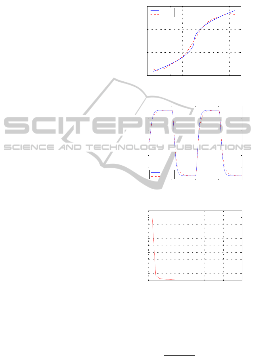
The algorithm shows promising results and mean

squared output error between normalized outputs of

actual and estimated systems converges to a ﬁnal

value of 4 × 10

−4

in 24 iterations of the algorithm.

Figure 3 shows the nonlinearity estimate. Conver-

gence of mean squared error is shown in Figure 5.

An easy way to evaluate the estimate of linear dy-

namic part lies in comparing the eigen values of the

estimated system with true ones. The eigen values of

the estimated system lie at

= 0.72,

= 0.53 and

= 0.53. Figure 4 shows the step response of the

dynamic linear part.

To evaluate the performance of the proposed al-

gorithm in noisy environment, zero mean Gaussian

additive noise is included at the output of the system

such that the signal to noise ratio (SNR) is 10dB. The

algorithm performs well in estimating the system de-

spite low output SNR. The ﬁnal mean squared error

converges to 1.4 × 10

−3

in 30 iterations. Nonlinear-

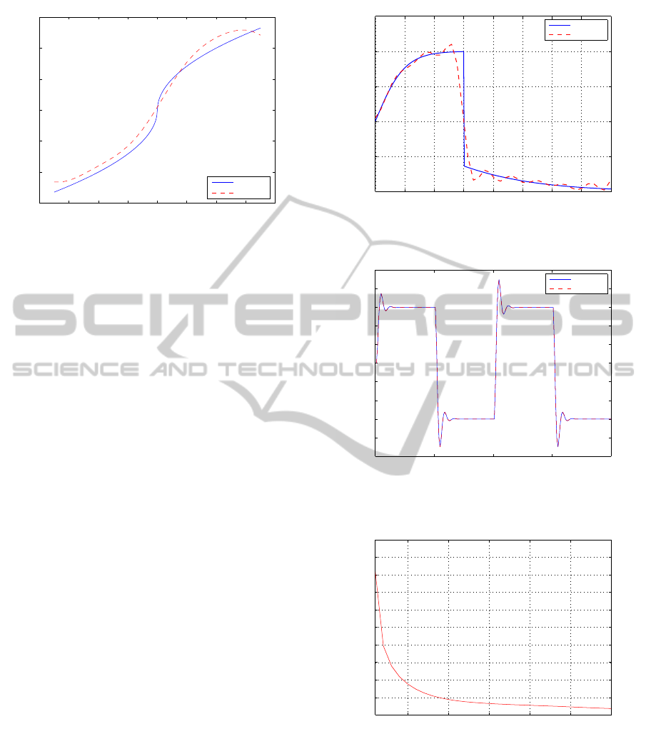
ity estimate is shown in Figure 6. The eigen values of

the estimated system lie at

10dB

= 0.73,

10dB

= 0.73

and

10dB

= 0.58.

The results presented above are obtained from a

single run of estimation algorithm. To further en-

sure the reliability and repeatability of the algorithm,

Monte-Carlo simulation is carried out and ensem-

ble statistics are tabulated in Table 1. The statistics

show encouraging convergence of normalized output

squared error and estimation of linear subsystem. Pa-

rameters of the nonlinearity cannot be compared be-

cause of the nonparametric nature of estimation. At

best, the estimates of nonlinearity can be judged from

the shapes of estimated nonlinear function as pre-

sented in Figures 3 and 6.

−2 −1.5 −1 −0.5 0 0.5 1 1.5 2

−1.5

−1

−0.5

0.5

1.5

Input

Output

Original

Estimated

Figure 3: Estimate of square root nonlinearity of example

0 50 100 150 200

−150

−100

−50

100

150

time samples

output

original

estimated

Figure 4: Step response of linear dynamic part of example

0 5 10 15 20 25

0.005

0.01

0.015

0.02

0.025

0.03

0.035

0.04

0.045

0.05

Iterations

Mean Squared Error

Figure 5: Mean squared error for example 1.

5.2 Example 2

The second example considers the following Ham-

merstein type nonlinear process whose static nonlin-

earity is given by

v(t) = tanh[2u(t)] 1.5 ≥ u(t),

v(t) =

exp(u(t)) − 1

exp(u(t)) + 1

4 > u(t) > 1.5.

NEURAL NETWORK BASED HAMMERSTEIN SYSTEM IDENTIFICATION USING PARTICLE SWARM

SUBSPACE ALGORITHM

185

Table 1: Monte-Carlo simulation statistics for example 1.

Estimation results without output noise

Total number of runs 200

Magnitude of actual eigen value λ

of linear subsystem 0.7

Mean magnitude of estimated eigen value

of linear subsystem 0.713

Variance of eigen value estimate

8× 10

−4

Magnitude of actual eigen value λ

of linear subsystem 0.6

Mean magnitude of estimated eigen value

of linear subsystem 0.62

Variance of eigen value estimate

4.5× 10

−3

Magnitude of actual eigen value λ

of linear subsystem 0.5

Mean magnitude of estimated eigen value

of linear subsystem 0.481

Variance of eigen value estimate

5.7× 10

−3

Average number of iterations required for every run 8.26

Average mean squared output error (MSE) 9.8× 10

−4

Estimation results with output SNR 10dB

Total number of runs 200

Magnitude of actual eigen value λ

of linear subsystem 0.7

Mean magnitude of estimated eigen value

of linear subsystem 0.75

Variance of eigen value estimate

1.6× 10

−3

Magnitude of actual eigen value λ

of linear subsystem 0.6

Mean magnitude of estimated eigen value

of linear subsystem 0.68

Variance of eigen value estimate

6× 10

−3

Magnitude of actual eigen value λ

of linear subsystem 0.5

Mean magnitude of estimated eigen value

of linear subsystem 0.4

Variance of eigen value estimate

6× 10

−2

Average number of iterations required for every run 8.02

Average mean squared output error (MSE) 6.6× 10

−3

The dynamic linear part is given by the following sec-

ond order discrete time state-space system

A =



1.0 1.0

−0.5 0.0



, B =



0.5



C =



1 0



The linear part of the system has eigen values at

1,2

= 0.5 ± 0.5i. Desired outputs are generated by

exciting the process model with a rich set of uni-

formly distributed random numbers in the interval

[0, 4]. An RBF network with 25 neurons is initial-

ized with random synaptic weights and uniformly dis-

tributed centers chosen within the input interval. PSO

social and cognitive parameters and constriction fac-

tor are kept similar to example 1. The number of par-

ticles is equal to the number of neurons and a popula-

tion size of 50 gives good results again. The algorithm

ICFC 2010 - International Conference on Fuzzy Computation

186

−2 −1.5 −1 −0.5 0 0.5 1 1.5 2

−1.5

−1

−0.5

0.5

1.5

input

output

original

estimated

Figure 6: Estimate of square root nonlinearity of example 1

with output SNR 10dB.

performs well and estimates the system in 20 itera-

tions. The mean squared output error between nor-

malized values of actual and estimated outputs con-

verges to a ﬁnal value of 8 × 10

−4

. The estimate of

nonlinearity shape is shown in Figure 7. Eigen val-

ues of the estimated system lie at

1,2

= 0.497± 0.5i.

Step response of linear subsystem is shown in Figure

8. The squared error convergence plot is shown in

Figure 9.

Estimation is then carried out in noisy environ-

ment, with zero mean Gaussian additive noise in-

cluded at the output of the system such that the sig-

nal to noise ratio (SNR) is 10dB. The algorithm per-

forms well in noisy environment. The ﬁnal mean

squared error converges to 1.8× 10

−3

in 30 iterations.

Nonlinearity estimate is shown in Figure 10. The

eigen values of the estimated system lie at

10dB

1,2

0.493± 0.499i.

Table 2 shows ensemble statistics of Monte-Carlo

simulation for example 2. The statistics show encour-

aging convergence of normalized output squared er-

ror and estimation of linear subsystem. As mentioned

before, parameters of the nonlinearity cannot be com-

pared due to the nonparametric nature of estimation.

At best, the estimates of nonlinearity can be judged

from the shapes of estimated nonlinear function as

presented in Figures 7 and 10.

6 CONCLUSIONS

The PSO/Subspace algorithm is basically a combi-

nation of PSO and Subspace N4SID algorithm, and

hence its convergence properties are directly related

to the convergence properties of PSO and Subspace

algorithms. PSO has been usually known to per-

form better than most evolutionary algorithms (EA)s

0 0.5 1 1.5 2 2.5 3 3.5 4

−1

−0.5

0.5

1.5

Input

Output

Original

Estimated

Figure 7: Estimate of tangent-hyperbolic nonlinearity of ex-

ample 2.

0 50 100 150 200

−5

−4

−3

−2

−1

time samples

output

original

estimated

Figure 8: Step response of linear dynamic part of example

5 10 15 20 25 30

0.8

1.2

1.4

1.6

1.8

2.2

2.4

2.6

2.8

x 10

−3

Iterations

Mean Squared Error

Figure 9: Mean squared error for example 2.

in ﬁnding global optimum provided its parameters are

tuned properly according to the application. The sub-

space algorithm is also known for having no conver-

gence problems. Its numerical robustness is guaran-

teed because of well understood linear algebra tech-

niques like QR decomposition and singular value de-

composition (SVD). As a consequence, it does not ex-

perience problems like lack of convergence,slow con-

NEURAL NETWORK BASED HAMMERSTEIN SYSTEM IDENTIFICATION USING PARTICLE SWARM

SUBSPACE ALGORITHM

187

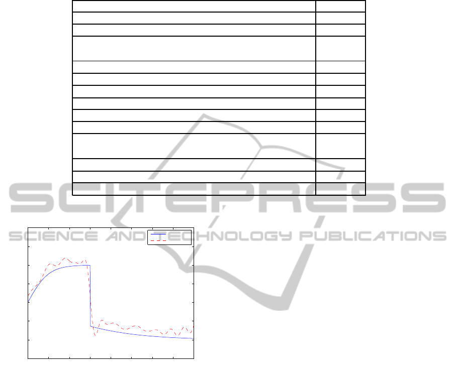
Table 2: Monte-Carlo simulation statistics for example 2

Estimation results without output noise

Total number of runs 200

Magnitude of actual eigen values λ

1,2

of linear subsystem 0.7071

Mean magnitude of estimated eigen values

1,2

of linear subsystem 0.7071

Variance of eigen value estimates 2× 10

−5

Average number of iterations required for every run 9

Average mean squared output error (MSE) 7× 10

−4

Estimation results with output SNR 10dB

Total number of runs 200

Magnitude of actual eigen values λ

1,2

of linear subsystem 0.7071

Mean magnitude of estimated eigen values

1,2

of linear subsystem 0.7079

Variance of eigen value estimates 6 × 10

−5

Average number of iterations required for every run 21

Average mean squared output error (MSE) 2 ×10

−3

0 0.5 1 1.5 2 2.5 3 3.5 4

−1.5

−1

−0.5

0.5

1.5

input

output

original

estimated

Figure 10: Estimate of tangent-hyperbolic nonlinearity of

example 2 with output SNR 10dB.

vergence or numerical instability (Overschee, P. V.,

Moor, B. D., 1994). Moreover, in order to assure re-

peatability and reliability of the proposed algorithm,

Monte-Carlo simulations have been carried out. The

ensemble statistics presented in Tables 1 and 2 show

strong convergenceand consistent performance of the

proposed algorithm.

The effect of noise is also studied, and the algo-

rithm is seen to converge sufﬁciently in the presence

of noisy data as shown in the simulation results.

ACKNOWLEDGEMENTS

The authors would like to acknowledge the support

of King Fahd University of Petroleum & Minerals,

Dhahran, Saudi Arabia.

REFERENCES

Abonyi, I., Nagy, L., Szeifert, E. (2000). Hybrid fuzzy con-

volution modelling and identiﬁcation of chemical pro-

cess systems. In International Journal Systems Sci-

ence. volume 31, pages 457-466.

Al-Duwaish, H. (2001). A genetic approach to the identiﬁ-

cation of linear dynamical systems with static nonlin-

earities. In International Journal of Systems Science.

volume 31, pages 307-314.

Al-Duwaish, H., Nazmulkarim, M., Chandrasekar, V.

(1997). Hammerstein model identiﬁcation by multi-

layer feedforward neural networks. In International

Journal Systems Science. volume 28, pages 49-54.

Billings, S. (1980). Identiﬁcation of nonlinear systems - a

survey. In IEE Proceedings. volume 127, pages 272-

285.

Carlisle, A., Dozier, G. (2001). An off-the-shelf pso. In

In Proceedings of the Particle Swarm Optimization

Workshop. pages 1-6.

Eberhart, R., Shi, Y. (1998). Parameter selection in particle

swarm optimisation. In Evolutionary Programming

VII. pages 591-600.

Eskinat, E., Johnson, S. H., Luyben, W. L. (1991). Use

of hammerstein models in identiﬁcation of nonlinear

systems. In AIChE Journal. volume 37, pages 255-

268.

Fruzzetti, K. P., Palazoglu A., McDonald, K. A. (1997).

Nonlinear model predictive control using hammer-

stein models. In J. Proc. Control. vol. 7, page 31-41.

Goethals, I., Pelckmans, K., Suykens, J. A. K., Moor, B. D.

(2005). Identiﬁcation of mimo hammerstein models

using least squares support vector machines. In Auto-

matica. volume 41, pages 1263-1272.

ICFC 2010 - International Conference on Fuzzy Computation

188

Greblicki, W. (1989). Non-parametric orthogonal series

identiﬁcation of hammerstein systems. In Interna-

tional Journal Systems Science. volume 20, pages

2335-2367.

Haddad, A. H., Thomas, J. B. (1968). On optimal and sub-

optimal nonlinear ﬁlters for discrete inputs. In lEEE

Transaction on Information Theory. volume 14, pages

16-21.

Haykin, S. (1999). Neural Networks - A Comprehensive

Foundation. Prentice-Hall, Second Edition.

Katayama, T. (2005). Subspace Methods for System Identi-

ﬁcation. Springer-Verlag, London.

Kennedy, J., Eberhart, R. (2001). Swarm Intelligence. Aca-

demic Press.

Luo, D., Leonessa, A. (2002). Identiﬁcation of mimo ham-

merstein systems with nonlinear feedback. In Pro-

ceedings of American Control Conference, Galesburg,

USA. pages 3666-3671.

Narendra, K. S., Gallman, P. (1966). An iterative method

for the identiﬁcation of nonlinear systems using ham-

merstein model. In IEEE Transaction on Automatic

Control. volume 11, pages 546-550.

Overschee, P. V., Moor, B. D. (1994). N4sid: Sub-

space algorithms for the identiﬁcation of combined

deterministic-stochastic systems. In Automatica. vol-

ume 30, pages 75-93.

V¨or¨os, J. (2002). Modeling and paramter identiﬁcation of

systems with multisegment piecewise-linear charac-

teristics. In IEEE Transaction on Automatic Control.

volume 47, pages 184-188.

Verhaegen, M., Westwick, D. (1996). Identifying mimo

hammerstein systems in the context of subspace

model identiﬁcation methods. In International Jour-

nal Control. volume 63, pages 331-349.

Wenxiao, Z. (2007). Identiﬁcation for hammerstein sys-

tems using extended least squares algorithm. In Pro-

ceedings of 26th Chinese Control Conference, China,.

pages 241-245.

Zhao, W., Chen, H. (2006). Recursive identiﬁcation for

hammerstein systems with arx subsystem. In IEEE

Transaction on Automatic Control. volume 51, pages

1966-1974.

NEURAL NETWORK BASED HAMMERSTEIN SYSTEM IDENTIFICATION USING PARTICLE SWARM

SUBSPACE ALGORITHM

189