
GRAPHLET DATA MINING OF ENERGETICAL INTERACTION
PATTERNS IN PROTEIN 3D STRUCTURES
Carsten Henneges, Marc R¨ottig
Center for Bioinformatics T¨ubingen, Eberhard Karls Universit¨at T¨ubingen, Sand 1, T¨ubingen, Germany
Oliver Kohlbacher, Andreas Zell
Center for Bioinformatics T¨ubingen, Eberhard Karls Universit¨at T¨ubingen, Sand 1, T¨ubingen, Germany
Keywords:
Graphlets, Data Mining, Relative Neighbourhood Graph, Secondary Structure Elements, Decision Tree Model
Selection
Abstract:
Interactions between secondary structure elements (SSEs) in the core of proteins are evolutionary conserved
and define the overall fold of proteins. They can thus be used to classify protein families. Using a graph
representation of SSE interactions and data mining techniques we identify overrepresented graphlets that can
be used for protein classification. We find, in total, 627 significant graphlets within the ICGEB Protein Bench-
mark database (SCOP40mini) and the Super-Secondary Structure database (SSSDB). Based on graphlets,
decision trees are able to predict the four SCOP levels and SSSDB (sub)motif classes with a mean Area Under
Curve (AUC) better than 0.89 (5-fold CV). Regularized decision trees reveal that for each classification task
about 20 graphlets suffice for reliable predictions. Graphlets composed of five secondary structure interactions
are most informative. Finally, we find that graphlets can be predicted from secondary structure using decision
trees (5-fold CV) with a Matthews Correlation Coefficient (MCC) reaching up to 0.7.
1 INTRODUCTION
Secondary structure elements (SSEs), β-sheets and
α-helices, are important building blocks of proteins
and interactions between these SSEs stabilize protein
tertiary structures. Many categorization schemes are
based on these SSEs like the SCOP (Murzin et al.,
1995) or CATH (Orengo et al., 1997) databases. For
example, the SCOP categorization scheme has four
levels, each one giving more detailed information
about the SSEs of a protein domain and the arrange-
ment of its SSEs.
An important question, especially in the context
of SSE-based categorization schemes like SCOP, is
whether there are interaction patterns between these
SSEs that occur preferably in native protein structures
or in protein structures of a given fold or superfamily.
As SSEs are complex three-dimensional structures,
whose relative states are hard to encode, analysing
the SSE interactions in full atomic detail can be-
come complex. However, encoding energetic inter-
action between SSEs as graphs makes this problem
amenable for graph-based analysis of protein struc-
tures. The SSEs of a structure are mapped to vertices
of a graph, and interactions between SSEs are repre-
sented by edges. Graph mining methods (Vacic et al.,
2010) can then be applied on these reduced represen-
tations of protein structures.
In the following sections, we mine these graph rep-
resentations for subgraphs, termed graphlets, that
preferably occur in native protein structures. The sig-
nificance of a graphlet is statistically tested using a
random graph model, serving as a background model
(Milo et al., 2002). This background model allows us
to identify graphlets that occur more often in protein
graphs than in random graphs. The value of the ex-
tracted graphlets is then demonstrated by using them
in predictors for SCOP levels and SSSDB motifs.
2 MATERIALS AND METHODS
Databases
We perform our experiments using protein struc-
tures from the SCOP40mini dataset from the ICGEB
database and the database of super-secondary struc-
190
Henneges C., Röttig M., Kohlbacher O. and Zell A..
GRAPHLET DATA MINING OF ENERGETICAL INTERACTION PATTERNS IN PROTEIN 3D STRUCTURES.
DOI: 10.5220/0003077501900195
In Proceedings of the International Conference on Fuzzy Computation and 2nd International Conference on Neural Computation (ICNC-2010), pages
190-195
ISBN: 978-989-8425-32-4
Copyright
c
2010 SCITEPRESS (Science and Technology Publications, Lda.)

tures SSSDB (Sonego et al., 2007; Chiang et al.,
2007).
Protein Preparation
We use C++ routines and the BALL library
(Kohlbacher and Lenhof, 2000) to analyse protein
structures. As a first step, hydrogen atoms are added.
After a consistency check of each residue, we assign
partial charges and atom radii to atoms according to
the AMBER force field. Finally, all hetero residues
are removed from the structure.
To be independent from protein annotation, all
SSEs are recomputed using the DSSP algorithm
(Kabsch and Sander, 1983), afterwards all residues
within loops are removed. α-helices are not further
modified, whereas all connected components of β-
strands linked by hydrogen bonds are merged into β-
sheets. In this way, each β-sheet is treated as a com-
plete 3D structure during the computation of interac-
tion energies.
Graphical Encoding of Energetic SSE
Interactions
To prepare the graph construction, we compute the
pairwise matrix of SSE interaction energies. Let A
and B be any secondary structures in a protein, and
let E[A, B, ...] be the AMBER energy of a set of SSEs,
then the pairwise interaction energy I[A, B] is given as
I[A, B] = E[A, B] − E[A] − E[B]. (1)
Graph construction serves for structural normal-
ization as well as extracting the interaction model.
It filters needless relations, while being independent
from the computed amount of I[A, B] energy and the
relative distance of the SSEs. Therefore, it makes pro-
teins having different numbers of SSEs comparable.
One convenient graph for this task is the Relative
Neighbourhood Graph (RNG) (Toussaint, 1980). The
RNG connects two labelled SSE nodes if the follow-
ing edge condition
I[A, B] ≤ max
C
{I[A,C], I[B,C]}, (2)
holds, where A, B,C are SSEs from the protein and
A 6= B 6= C. The RNG is a connected proximity graph
and, therefore, also connects SSEs that are too distant
for direct protein residue contacts. As its edge con-
dition resembles an ultra-metric (Milligan and Isaac,
1980), the RNG has shown great robustness in prac-
tice and is a powerful tool to extract meaningful per-
ceptual structures (Toussaint, 1980).
Graphlet Analysis
Graphlet analysis makes use of subgraph sampling
and, therefore, relies on a graph isomorphism test.
Each sampled subgraph is referred to as graphlet and
its frequency or probability within a network is esti-
mated by repeated sampling. In addition, statistical
graphlet analysis requires the knowledge of a back-
ground distribution to compute the probability of an
observation. As no analytical distribution function for
graphlets is known, their probabilities are in general
estimated from random graphs.
To obtain a random model resembling the input
graph distribution, each protein graph is randomized.
We use a random rewiring method where each edge
is split into two half-edges. Then, all half-edges are
randomized and rewired. This is repeated until a con-
nected graph is obtained or a maximum number of
iterations is reached. In the latter case, the last sam-
ple is saved. In summary, random rewiring conserves
important graph properties (e.g. the node degree). By
randomizing each graph once, we obtain a collection
of random graphs that closely resembles the test dis-
tribution.
Next, we estimate the graphlet distribution by ran-
dom sampling connected subgraphs. The goal of
the sampling is twofold: First, all existent graphlets
should be detected and, second, their distribution
should be estimated correctly. If all graphlets were
known in advance, drawing a fixed number of samples
would yield the maximum likelihood estimate of the
graphlet distribution, which is a multinomial distribu-
tion (Wassermann, 2004; Georgii, 2004). To achieve
this estimate, we employ a two-pass approach for this
task.
In the first pass, the data is exploratory sampled.
For counting the graphlet frequencies, we make use
of a Move-to-Front (MF) list that holds a counter for
each graphlet type. Thus, each sampled graphlet is
first searched in the MF list for counting its occur-
rence and inserted in the case it is not found. There-
fore, the MF list length increases during this pass. We
draw 1000 samples per graph of the database to min-
imize the possibility of missing patterns.
In the second pass, we keep the MF list fixed dur-
ing sampling to compute the maximum likelihood es-
timates. Again, we draw a total of 1000 samples, 5
repetitions with 200 samples, from each graph and,
thus, obtain 5 independent distribution estimates. If
sampling detects an unknown graphlet within the sec-
ond pass, a counter for unknownpatterns is increased.
Finally, we compute the distribution estimate by aver-
aging and normalizing all samplings for a graph.
We choose a sampling size of 1000 graphlets in
GRAPHLET DATA MINING OF ENERGETICAL INTERACTION PATTERNS IN PROTEIN 3D STRUCTURES
191

each phase because only a small fraction of the RNG
comprises more than 40 nodes, i.e., only a small frac-
tion of the database proteins are large. As the number
of graphlets increases exponentially with pattern size,
a trade-off between estimation accuracy and runtime
is required. We found that a sampling size of 1000 is
sufficient to accurately estimate the graphlet distribu-
tion within a reasonable runtime.
To determine significant graphlets, we employ
permutation testing, which is a non-parametric tech-
nique to efficiently test the equality of two distribu-
tions g, h (Wald and Wolfowitz, 1944). It requires no
assumptions on the true probability distributions. By
resampling new random distributions from the input
distribution and evaluating a test statistic T, it infers
the distribution of T under H
0
: g = h. This denotes
the case where g and h are equal and, therefore, al-
lows to compute the p-value for the hypothesis that
the input distributions are equal. In our experiments,
we use the
coin
package implemented in
R
(R Devel-
opment Core Team, 2009).
For each graphlet, we employ permutation testing
to compute the likelihood that its distribution on the
protein graphs equals its distribution on the random-
ized graphs. Hence, we determine those graphlets that
are significantly over or under-represented in random
graphs. To account for the multiple-testing problem,
we afterwards adjust the p-values according to the
method of (Holm, 1979). Finally, all graphlets be-
low a significance threshold of 0.05 and having a fre-
quency ratio at least 10-fold larger on protein graphs
than on the random graphs are retained for further
analysis. Figure 1 illustrates this analysis step.
Figure 1: The graphlet analysis workflow using a random
control and permutation testing.
Decision Tree Analysis
Here, we relate the extracted graphlets to global pro-
tein structure properties, e.g. the SCOP classifica-
tion of each structure. Therefore, we employ decision
trees as they facilitate a better understanding of the
data set. Inspection of leafs and their associated sam-
ples allows relating specific graphlets to proteins and,
thus, facilitates the analysis of structures with respect
to interaction patterns. In addition, decision trees are
native multi-class prediction algorithms and are thus
a convenient choice for the prediction of various pro-
tein classes. However, decision trees tend to overfit
and therefore require careful complexity regulariza-
Table 1: Results of the Graphlet Analysis.
Graphlet Found Significant Filter
Size Graphlets Graphlets Ratio
4 427 22 0.05
5 1,731 77 0.04
6 5,366 212 0.04
7 16,904 316 0.02
tion.
An alternative to decision trees are neural network
predictors. Neural networks represent a non-linear
class of regression functions that are estimated by gra-
dient descent. For each class a single output neu-
ron can be integrated into the network and, thus, a
single neural network can model the posterior proba-
bility of each class using a common basis of hidden
neurons. However, neural networks are pure highly
non-linear prediction models and, therefore, hard to
interpret. Consequently, they are less suited for data
mining purposes and do not provide much insight into
the dataset.
Using the graphlet distributions, we encode each
protein as a binary vector of graphlet occurrences.
Whenever a graphlet is found for a protein, it is en-
coded as 1 and as 0 else. In addition, we integrate the
SCOP level information from ICGEB as well as the
SSSDB Motif class information as a prediction target.
SCOP has four hierarchical levels: the class, fold, su-
perfamily and family of a protein domain. Similarly,
the SSSDB Motif Class encodes the super-secondary
structure super class, while the SSSDB Motif Sub-
class denotes a more precise subdivision.
We use the
partition
platform from
JMP
(SAS
Institute Inc., 2009) for learning. JMP is a reduced
version of the SAS Enterprise Miner software suite,
which is extensively used for professional data anal-
ysis in industry, and provides various platforms that
facilitate data analysis tasks. Especially, the ability of
the
partition
platform to easily inspect each predic-
tion node is helpful during the analysis of the inferred
graphlets. In our experiments, the Minimum Split
Size (MSS) parameter is chosen to be 5, 10, 15, 20, 25
and 50, while training on graphlets of size 4 to 7. For
each model, the prediction performance is evaluated
using 5-fold cross-validation to compute AUC values
for each class. Then, all AUC values are averaged to
yield the mean AUC (mAUC) for each combination
of graphlet size and MSS. For comparison purposes,
we also employ the
neural nets
platform.
Regularization
However, to obtain regularized decision trees, we fol-
low the work of (Scott and Nowak, 2005). There, the
ICFC 2010 - International Conference on Fuzzy Computation
192

space of decision tree hypotheses is regularized by
their number of leafs and their prediction error. Let T
be the hypothesis space of decision trees and |T| de-
note the number of leafs of a tree T. Furthermore, let
n be the number of data samples and λ be a weighting
factor between tree complexity and prediction error,
then the Complexity Regularization CR for decision
tree selection is given as
CR = argmin
T
ˆ
R
|{z}
Empirical risk
+λ
r
|T|
n
|{z}
Bound on bias
(3)
where
ˆ
R denotes the prediction error and n the num-
ber of training samples. In our case, we set
ˆ
R =
1 − mAUC, because we are dealing with multi-class
predictions and the mAUC is a performance measure
between 0 and 1 that can be converted into an error
by subtracting it from 1. This error is then compared
to its theoretical bound, the Uniform Deviation Bound
UDB
n
, which upper bounds the true risk of a decision
tree and is given as
UDB
n
= argmin
T∈T
(
ˆ
R(T) +
r
3|T| + log(n)
2n
)
. (4)
The remaining task is to find a valid λ for regular-
ization. We choose λ to minimize
λ = argmin
λ
∑
T
(CR −UDB
n
)
2
(5)
for all considered decision trees, trained with MSS of
5, 10, 15, 20, 25, and 50.
3 RESULTS & DISCUSSION
Graphlet Extraction
We convert 1357 proteins from the ICGEB
SCOP40mini database and 744 proteins from
the SSSDB into the described graphical representa-
tion. Figure 2 illustrates the result of a conversion.
This results in a total of 2101 graphs left for graphlet
analysis. Two other datasets from ICGEB, PCB00020
(11,944 structures from SCOP95) and PCB00026
(11,373 structures from CATH95), are convenient for
our experiments. However, the enormous number of
graphlets found in this data sets leads to infeasible
computation times. Therefore, we restrict our analy-
sis to the smallest ICGEB collection and included the
SSSDB instead.
Table 1 summarizes our sampling results. It
shows that increasing the graphlet pattern size also
Figure 2: Structure (left) and RNG (right) of ICGEB struc-
ture
d1pmma
. Box nodes denote β-sheets, whereas round
nodes refer to α-helices.
increases the number of detected graphlets as well
as the number of significant graphlets. However, the
ratio between significant and detected graphlets re-
mains below 5%. Hence, we extract only a small
amount of significant patterns from a large collection
of graphlets (see Table 1).
Decision Tree Learning
For each target variable the decision tree minimizing
CR −UDB
n
is selected as the regularized model and
saved for final analysis. We find that λ = 1.3 fulfills
equation (5) for each target variable. We choose λ
such that the total squared deviation from the UDB
n
was minimal when averaged over all models using
any size of graphlets and any number of splits. Conse-
quently, all models are regularized and have maximal
expressive power along with a reduced probability of
overfitting. Table 2 lists the MSS, graphlet size, num-
ber of splits, as well as the mAUC of the final models
for each target variable. We find that simple models
suffice to achievemAUC better than 0.82. In addition,
at least 20 samples can be summarized in a leaf to re-
sult in a decision tree predicting one category without
sacrificing prediction performance. Finally, we find
that graphlets of size 5 are in most cases superior to
others. Also graphlets of size 4 and 7 are used for
decision tree learning and, therefore, provide useful
information (Table 2).
We also compare the performance of decision
trees to the performance of neural networks, also im-
plemented in JMP. The last column of Table 2 shows
the mean AUC achieved by the
neural nets
plat-
form using cross-validation on a random selection of
40% of the samples, which are held out as external
validation set. The platform was trained using the de-
fault values. We find that the neural network is supe-
rior to our regularized decision trees in predicting the
SCOP class and SCOP family, as well as the SSSDB
Motif Class. However, the performance difference
does not exceed a value of 0.06 mAUC points. Con-
GRAPHLET DATA MINING OF ENERGETICAL INTERACTION PATTERNS IN PROTEIN 3D STRUCTURES
193
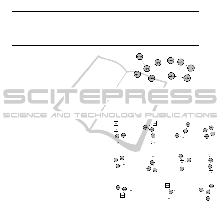
Table 2: Regularized Decision Trees for each target variable.
Target Variable # classes Graphlet MSS Performed mAUC Neural Net
Size Splits mAUC
SCOP class 5 5 20 23 0.87 0.92
SCOP fold 19 5 20 24 0.87 0.84
SCOP superfamily 7 4 20 24 0.85 0.83
SCOP family 48 5 20 16 0.83 0.87
SSSDB Motif Class 32 7 10 22 0.93 0.99
SSSDB Motif Subclass 153 5 15 21 0.96 0.96
sequently, decision trees and neural networks achieve
a comparable performance and, therefore, support the
descriptive value of our graphlet features.
Next, we extract all graphlets from the selected
regularized decision tree models to analyse their us-
ages with respect to all target variables. Here, we find
graphlets that are used several times for the predic-
tion of various target variables, while other graphlets
are specific to one class.
While 66 graphlets are used only for the prediction
of one target variable, we find two graphlets of size
5 that are used to predict 4 different target variables
(Figure 3). Note that this is the maximum number
achievable because two target variables are predicted
using graphlets of size 4 and 7.
In Figure 4 all SCOP superfamily graphlets are
shown. Within the decision tree for the SCOP super-
family, the graphlets (a) and (b) in Figure 4 are more
relevant for classification, because they are used in
three and two splits, respectively. Interestingly, (a)
and (b) are paths of helices containing one or two
sheets, while the other graphlets consist mainly of star
topologies.
Finally, we predict all detected graphlets from sec-
ondary structure sequence. Therefore, we convert
each protein sequence into strings of symbols h,s, l
encoding whether a residue is within a helix, strand
or loop. We design a set of 439 features describing
lengths, as well as densities, normalized to protein
length, of helices, strands, loops. In addition, we de-
sign regular expressions for SSE sequence patterns,
which result in binary features. Then, we train deci-
sion trees, implemented in the
rpart
package of
R
,
and use 5-fold cross-validation using the
bootstrap
package to estimate the MCC (Baldi et al., 2000). We
find that chains of SSEs and star topologies can be
best predicted by decision trees.
4 CONCLUSIONS
In summary, we find that significantly overrepre-
sented patterns in energetic SSE interactions exist and
(a) (b)
Figure 3: Graphlet 3(a) predicts 4 targets and is predictable
with MCC=0.6, while graphlet 3(b) predicts 4 targets and is
predictable with MCC=0.5 from secondary-structure infor-
mation.
Figure 4: This figure shows all extracted graphlets used for
the prediction of the SCOP superfamily.
can be found using graphlet analysis. Regularized
decision tree learning on the mined patterns predicts
SCOP levels and SSSDB Motifs with great accuracy
(mAUC > 0.8) using about 20 graphlets. Also, the
presence of a specific graphlet can be predicted from
secondary structure sequence of a protein with MCC
values up to 0.7. Finally, we demonstrate that the
combination of graphlet analysis using permutation
testing and decision tree learning facilitates automatic
categorization of protein structures.
We have shown that graphlets are predictable from
the secondary structure sequence, therefore graphlets
can be used as constraints for the placement of pre-
dicted secondary structure elements, when predict-
ICFC 2010 - International Conference on Fuzzy Computation
194

ing the tertiary structure from the protein sequence
alone. Thus, future work should focus on the usage of
the predictable graphlets to improve ab initio protein
structure prediction.
REFERENCES
Baldi, P., Brunak, S., Chauvin, Y., Andersen, C. A. F., and
Nielsen, H. (2000). Assessing the accuracy of predic-
tion algorithms for classification: an overview. Bioin-
formatics, 16(5):412–424.
Chiang, Y.-S., Gelfand, T. I., Kister, A. E., and Gelfand,
I. M. (2007). New classification of supersecondary
structures of sandwich-like proteins uncovers strict
patterns of strand assemblage. Proteins, 68(4):915–
921.
Georgii, H.-O. (2004). Stochastik. de Gruyter, 2nd edition.
p.198.
Holm, S. (1979). A simple sequentially rejective multi-
ple test procedure. Scandinavian Journal of Statistics,
6(2):65–70.
Kabsch, W. and Sander, C. (1983). Dictionary of protein
secondary structure: Pattern recognition of hydrogen-
bonded and geometrical features. Biopolymers,
22(12):2577–2637.
Kohlbacher, O. and Lenhof, H.-P. (2000). BALL–rapid soft-
ware prototyping in computational molecular biology.
Bioinformatics, 16(9):815–824.
Milligan, G. W. and Isaac, P. D. (1980). The validation of
four ultrametric clustering algorithms. Pattern Recog-
nition, 12(2):41 – 50.
Milo, R., Shen-Orr, S., Itzkovitz, S., Kashtan, N.,
Chklovskii, D., and Alon, U. (2002). Network Mo-
tifs: Simple Building Blocks of Complex Networks.
Science, 298(5594):824–827.
Murzin, A. G., Brenner, S. E., Hubbard, T., and Chothia,
C. (1995). Scop: A structural classification of pro-
teins database for the investigation of sequences and
structures. Journal of Molecular Biology, 247(4):536
– 540.
Orengo, C. A., Michie, A. D., Jones, S., Jones, D. T.,
Swindells, M. B., and Thornton, J. M. (1997). CATH–
a hierarchic classification of protein domain struc-
tures. Structure, 5(8):1093–1108.
R Development Core Team (2009). R: A Language and
Environment for Statistical Computing. R Foundation
for Statistical Computing, Vienna, Austria. ISBN 3-
900051-07-0.
SAS Institute Inc. (2009). Jmp 8.0.1. www.jmp.com.
Scott, C. and Nowak, R. (2005). On the adaptive properties
of decision trees. In Advances in Neural Information
Processing Systems 17. MIT Press.
Sonego, P., Pacurar, M., Dhir, S., Kertesz-Farkas, A., Koc-
sor, A., Gaspari, Z., Leunissen, J. A. M., and Pon-
gor, S. (2007). A Protein Classification Benchmark
collection for machine learning. Nucleic Acids Res,
35(Database issue):D232–D236.
Toussaint, T., G. (1980). The relative neighbourhood graph
of a finite planar set. Pattern Recognition, 12:261 –
268.
Vacic, V., Iakuoucheva, L., Lonardi, S., and Radivojac, P.
(2010). Graphlet kernels for prediction of functional
residues in protein structures. Journal of Computa-
tional Biology, 17(1):55 – 72.
Wald, A. and Wolfowitz, J. (1944). Statistical tests based
on permutations of the observations. The Annals of
Mathematical Statistics, 15(4):358–372.
Wassermann, L. (2004). All of statistics. Springer. theorem
14.5.
GRAPHLET DATA MINING OF ENERGETICAL INTERACTION PATTERNS IN PROTEIN 3D STRUCTURES
195
