SYSTEM IDENTIFICATION BASED ON MULTI-KERNEL LEAST
SQUARES SUPPORT VECTOR MACHINES
(MULTI-KERNEL LS-SVM)
Mounira Tarhouni, Kaouther Laabidi, Moufida Lahmari-Ksouri
Unit of Research Analysis and control of systems (ACS, ENIT), BP 37, Le Belvedere 1002, Tunis, Tunisia
Salah Zidi
LAGIS (USTL, Lille), Villeneuve d’Ascq, 59650 Lille, France
Keywords:
Nonlinear system identification, Least Squares Support Vector Machines (LS-SVM), Multi-kernel function,
Multi model, Weighted function.
Abstract:
This paper develops a new approach to identify nonlinear systems. A Multi-Kernel Least Squares Support
Vector Machine (Multi-Kernel LS-SVM) is proposed. The basic LS-SVM idea is to map linear inseparable
input data into a high dimensional linear separable feature space via a nonlinear mapping technique (kernel
function) and to carry out linear classification or regression in feature space. The choice of kernel function
is an important task which is related to the system nonlinearity degrees. The suggested approach combines
several kernels in order to take advantage of their performances. Two examples are given to illustrate the
effectiveness of the proposed method.
1 INTRODUCTION
In the field of automatic control, obtaining an accu-
rate model of dynamical system is an important task
that can influence the overall performance of the con-
trol loop (Lauer, 2008). System identification aims at
finding such an appropriate model of the system based
on preliminary equations and input/output data. The
model can be classified on three types: White Box
models, Grey Box models and Black Box models,
the last one is considered when no physical insight
is available nor used (Lauer, 2008).
Recently, a new kind of learning machine called Sup-
port vector machines (SVM) has been presented and
used for classification (Zidi et al., 2006), (Diosan
et al., 2007), (ElFerchichi et al., 2009), (Tarhouni
et al., 2010) and for regression (Lauer, 2008). The
basic idea is to map linear inseparable input data into
a high dimensional linear separable feature space via
a nonlinear mapping technique (kernel function) and
to carry out linear classification or regression in fea-
ture space.
Recent developments in the literature on the SVM
have emphasized the need to consider multiple ker-
nels based learning method (Lanckriet et al., 2004),
(Zhejing et al., 2004), (Sonnenburg et al., 2006) and
(Diosan et al., 2007). This idea reflects the fact
that practical learning problems often involve mul-
tiple, heterogeneous data sources. (Diosan et al.,
2007) have developed an Evolved Combined Kernels
(ECKs). They have considered a combination of mul-
tiple kernels and they have used a genetic algorithm
(GA) for evolving these weights. This proposed ap-
proach is used for solving classification problems.
They have compared their results against those ob-
tained by (Lanckriet et al., 2004) with a combined
kernel learnt with convex methods (CCKs).
A variant of SVM called Least Squares Support Vec-
tor Machines (LS-SVM) method has been developed
as an attractive tool for identification of complex non
linear systems (Suykens and J.Vandewalle, 1999).
This method is a widely known simplification of the
SVM, allowing to obtain the model by solving a sys-
tem of linear equations instead of a hard quadratic
programming problem involved by the standard SVM
(Valyon and Horvath, 2005). It is empirically found
that the LS-SVM method yields a similar perfor-
mance compared to the classical SVM on classifica-
tion problems, and often outperforms SVM in the re-
gression case.
310
Tarhouni M., Laabidi K., Lahmari-Ksouri M. and Zidi S..
SYSTEM IDENTIFICATION BASED ON MULTI-KERNEL LEAST SQUARES SUPPORT VECTOR MACHINES (MULTI-KERNEL LS-SVM).
DOI: 10.5220/0003077703100315
In Proceedings of the International Conference on Fuzzy Computation and 2nd International Conference on Neural Computation (ICNC-2010), pages
310-315
ISBN: 978-989-8425-32-4
Copyright
c
 2010 SCITEPRESS (Science and Technology Publications, Lda.)

The LS-SVM method proved its efficiency in nu-
merous application fields such as classification (Tao
et al., 2009), identification of hybrid system (Lauer,
2008), identification of MIMO Hammerstein system
(Goethals et al., 2005) ···.
On the last decades, LS-SVM has been applied in
the field of predictive control. (Zhejing et al., 2007)
have developped a nonlinear model predictive control
based on Support Vector Machine with Multi-kernel,
where a nonlinear model can be transformed to linear
model. They have used a model of a SVM with linear
kernel followed in series by a SVM with spline ker-
nel function. In the same context, (Lei et al., 2008)
propose an on-line predictive control based on LS-
SVM and they have demonstratethat their method has
enough rapid speed to establish an on-line model and
strong robustness to external disturbance and param-
eters variation.
Although the advantages of regression task based on
LS-SVM approach are considerable, this approach is
often confronted to the problem of choice of an ap-
propriate kernel functions and the choice of these pa-
rameters.
In this paper, our main contribution is the proposition
and the application of a new Multi kernel LS-SVM
identification method. Indeed, our idea consists on
the combination of multiple kernel function in order
to take advantage of their performances. In this con-
text, we have chosen a linear kernel function which
it is very performant in the identification task and we
havecombined the Gaussien kernel to predict the non-
linearity in the system behaviour. The performances
of this approach are illustrated through the identifica-
tion of two nonlinear benchmarks.
This paper is organized as follows. In Section 2, the
method ”least squares Support Vectors Machines” is
presented. In Section 3, a description of the proposed
identification method based on multi kernel LS-SVM
is given. A numerical example to illustrate the proper-
ties of the proposedmethod in the case of multi-model
system is investigated in Section 4.
2 LEAST SQUARES SUPPORT
VECTOR MACHINES (LS-SVM)
(Suykens and J.Vandewalle, 1999) have presented the
LS-SVM approach, in which the following function ϕ
is used to approximate the output system as follows:
y =< w, ϕ(x) > +b (1)
where x ∈ ℜ
m
are the input data, y ∈ ℜ are the output
data and ϕ(.) :ℜ
m
7→ℜ
n
k
is the nonlinear function that
maps the input space into a higher dimension feature
space.
LS-SVM approach was defined in the following con-
strained optimization problem .



min
w,b,e
J
P
(w, e) =
1
2
kwk
2
2
+C
1
2
∑
N
i=1
e
2
i
subject to : y
i
=< w, ϕ(x
i
) > +b + e
i
k = 1, 2, ··· , N
(2)
Where e
i
are slack variable and C is a regularization
factor.
The corresponding Lagrangian involving the dual
variables α
i
is described by relation (3).
L(w, b, e, α) = J
p
(w, e)−
N
∑
i=1
α
i
(< w, ϕ(x
i
) > +b+ e
i
−y
i
)
(3)
Where α
i
are lagrange multipliers. The optimality
conditions are:





∂l
∂w
= 0 7→ w =
∑
N
i=1
α
i
ϕ(x
i
)
∂L
∂b
= 0 7→
∑
N
i=1
α
i
= 0
∂l
∂e
i
= 0 7→ α
i
= Ce
i
, k = 1, ··· , N
(4)
By replacing the expression of w and e
i
in the opti-
mization problem constraints (2), We obtain:
y
i
=
N
∑
j=1
α
j
< ϕ(x
i
), ϕ(x
j
) > +b+
1
C
α
i
(5)
The parameters are recovered as solution of the fol-
lowing linear system:
"
0
−→
1
T
−→
1 Ω+C
−1
I
#

b
α

=

0
y

(6)
Where Ω = ϕ(x
i
)
T
ϕ(x
j
) = k(x
i
, x
j
) is the kernel ma-
trix.
Using LS-SVM approach the output model will be
given by relation (7).
y(x) =
N
∑
i=1
α
i
K(x, x
i
) + b (7)
Where α
i
, b ∈ ℜ are the solution of equation (6), x
i
is
training data and x is the new input vector.
3 SYSTEM IDENTIFICATION
BASED ON MULTI-KERNEL
LS-SVM
The identification diagram structure based on LS-
SVM is shown in figure 1. Where y(k) is the actual
plant output and ˆy(k) is the estimated output.
SYSTEM IDENTIFICATION BASED ON MULTI-KERNEL LEAST SQUARES SUPPORT VECTOR MACHINES
(MULTI-KERNEL LS-SVM)
311

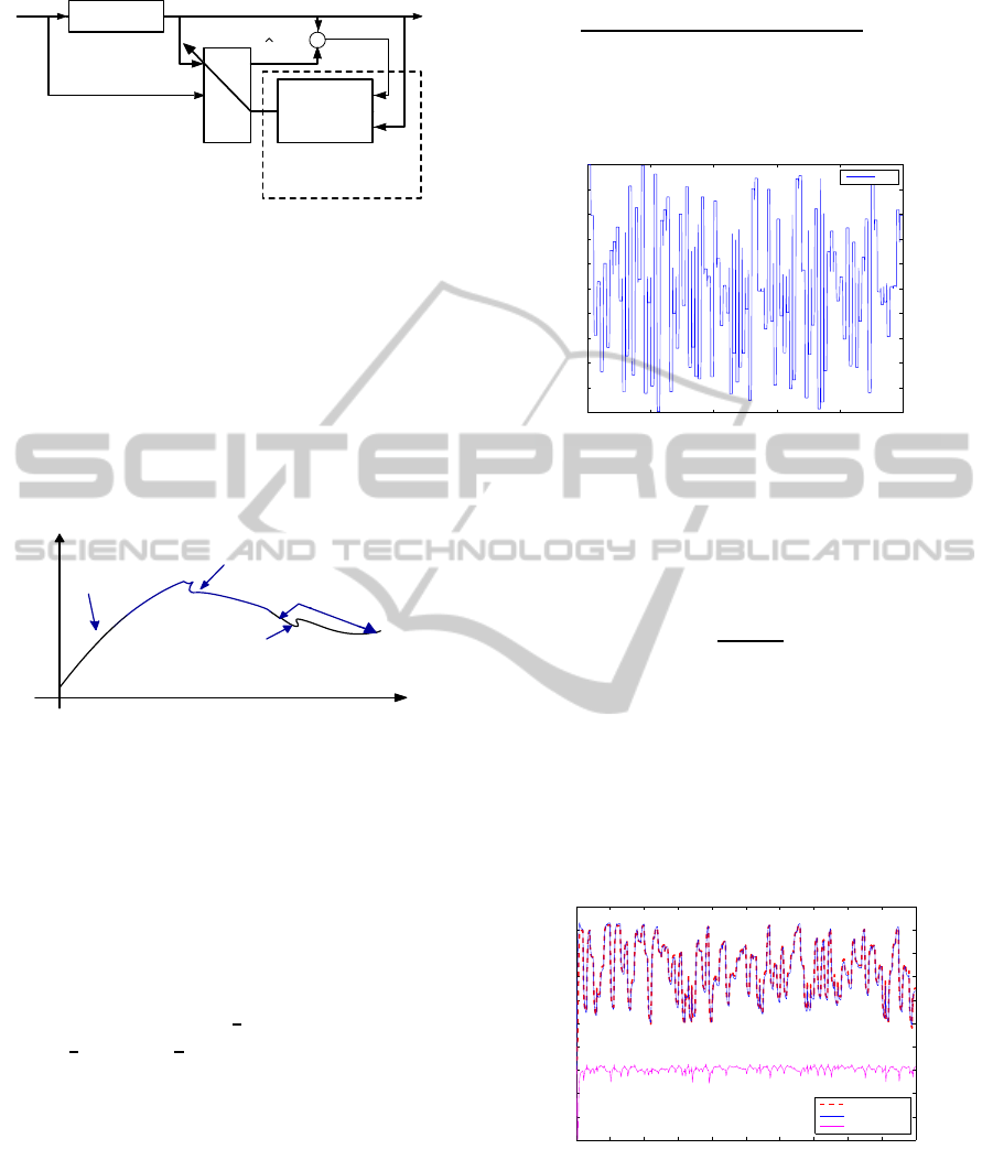
Plant
u(k) y(k)
+
-
Training
algorithm
LS-SVM model
y(k)
Choice of the
Kernel Function
Figure 1: Identification structure based on LS-SVM.
The LS-SVM model output is based on lagrange mul-
tipliers and kernel function K(x
i
, x). The lagrange
multipliers were generated by resolving the equation
system (6). These lagrange multipliers depend also on
the kernel matrix k(x
i
, x
j
). Hence, the choice of this
function is a crucial task. In this note, the proposed
kernel is obtained by combining a linear kernel and a
nonlinear one that will be used successively to iden-
tify the linear and the nonlinear parts as shown Figure
2.
gaussien
kernel
linear kernel
linear kernel
gaussien
kernel
y
Time
system output
Figure 2: multi-kernel LS-SVM principle.
The provided idea is explained by the following de-
velopement.
We suppose that our output will be expressed by two
weighted functions ϕ
1
and ϕ
2
.
y = a
1
< w
1
, ϕ
1
(x) > +a
2
< w
2
, ϕ
2
(x) > +b (8)
Where a
1
and a
2
are the weighting factors.
In this case, the new optimisation problem formula-
tion is given by these constraints:











min
w,b,e
J
P
(w, e) =
1
2
kw
1
k
2
2
+
1
2
kw
2
k
2
2
+C
1
2
∑
N
i=1
e
2
i
subject to : y
i
= a
1
< w
1
, ϕ
1
(x) > +
a
2
< w
2
, ϕ
2
(x) > +b+ e
i
i = 1, 2, ···, N
(9)
Using the steps given in section (2). The output will
be rewrited as follows:
y =
N
∑
i=1
α
i
(a
1
K
1
(x, x
i
) + a
2
K
1
(x, x
i
)) + b (10)
To illustrate the effectiveness of our proposed method,
we consider the following single-input/single-output
(SISO) system (Verdult et al., 2002):
y(k) =
y(k−1)y(k−2)(y(k−1) + 4.5)
1+ y(k−1)
2
+ y(k−2)
2
+ u(k−1)
(11)
With an input excitation signal chosen as a multiple
square signal represented in figure 3.
0 200 400 600 800 1000
−1
−0.8
−0.6
−0.4
−0.2
0
0.2
0.4
0.6
0.8
1
u(k)
Figure 3: command signal.
We generate a 1000 patterns, the first 500 samples are
used as training test and the remaining 500 samples
are used to validate the obtained model.
The fitness criterion (Bemporad et al., 2005):
FIT = (1−
kˆy−yk
ky− ¯yk
) ×100% (12)
is used to measure the similarity between the real out-
put system y = [y(1)···y(N)]
T
and the estimated out-
put ˆy = [ˆy(1)··· ˆy(N)]
T
. ¯y is the average of measure-
ments y(k), k = 1,···, N. Where N is the number of
available measurement points.
The training LS-SVM algorithm has as input the vec-
tor x = [u(k) u(k−1) y(k −1) y(k −2) y(k −3)]
T
and
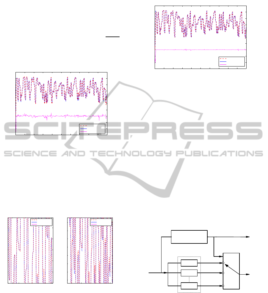
as output y(k). Figure 4 shows the system output
0 100 200 300 400 500 600 700 800 900 1000
−3
−2
−1
0
1
2
3
4
5
6
7
System output
Model output
Identification error
Figure 4: Identification based on LS-SVM with linear ker-
nel.
and the LS-SVM model based on a linear kernel.
We have considered a polynomial kernel function
k(x, y) = (x
T
y + cst)
n
. To determine the appropriate
parameters, we have considered several test valida-
tion. We have fixed : cst=120, n=1, the optimisation
ICFC 2010 - International Conference on Fuzzy Computation
312

parameter C is taken equal to 5 and we obtain a FIT
criterion equal to 82.40%
To compare the obtained results using linear kernel
with these obtained using the Gaussian one. We have
considered a gaussian kernel: K(x, y) = exp(−
kx−yk
2
2σ
2
)
Its kernel parameter is selected by cross validation.
The bandwidth σ value is equal to 1 and the regular-
ization parameter C is also, taken equal to 5. Then,
the FIT converges to 80.95% .
0 100 200 300 400 500 600 700 800 900 1000
−3
−2
−1
0
1
2
3
4
5
6
7
System output
Model output
Identification error
Figure 5: Identification based on LS-SVM with Gaussian
kernel.
We conclude that, the identification based on LS-
SVM with linear kernel is more accurate than with
Gaussian kernel in this case. However, curve peaks
are identified using the Gaussian kernel better than the
linear one as shown in Figure 6. This figure represents
an enlarged part of the simulations results obtained by
the tow last LS-SVM model.
350 400 450 500 550 600 650
3.8
4
4.2
4.4
4.6
4.8
System output
Model output
Identification error
300 400 500 600 700
3.6
3.8
4
4.2
4.4
4.6
4.8
5
System output
Model output
Identification error
Figure 6: Identification based on LS-SVM with: polyno-
mial kernel (right), Gaussian kernel (left).
For this purpose, we propose to combine the both ker-
nels and to generate a Multi Kernel LS-SVM method
to identify the system behaviour. So, the candidate
kernel is composed by linear and Gaussian kernels.
The two kernels were weighted by two parameters a
1
and a
2
fixed successively to 0.7 and 0.3. These param-
eters were selected after several tests. a
1
is greater
than a
2
. This choice is justified, indeed the identifi-
cation results using linear kernels are better than the
Gaussian one.
0 100 200 300 400 500 600 700 800 900 1000
−3
−2
−1
0
1
2
3
4
5
6
7
System output
Model output
Identification error
Figure 7: Multi-kernel LS-SVM identification.
The obtained identification result are presented in
the figure 7. We notice that the real system output and
the model output are overcome. The FIT criterion is
taken equal to 88.64% witch is better than the crite-
rion obtained with the last two methods.
3.1 Identification of Multimodel System
based on Multi-kernel LS-SVM
When the complexity of the plant increases the tra-
ditional methods of modeling prove, often, incom-
petent to generate a global model likely to give an
account of all the system characteristics. The multi-
model approach was developed to bring an answer to
these problems (Messaoud et al., 2009), (Zouari et al.,
2008). This approach consists to represent the process
by several models .
The multi model identification based on our proposed
method is shown in the following diagram 8:
Kernel 2
Kernel C
u(k)
y(k)
library of model
y
y
y
1
2
C
Plant
validity
calculation
Kernel 1
m
m
m
1
C
2
Figure 8: Multimodel structure identification based on
Multi kernel LS-SVM.
The idea proposed in this case is to construct a
library of models. Every operating domain is iden-
tified using the proposed Multi-kernel LS-SVM ap-
proach. The parameters of the kernel function and
the weighting factors are different from model to an
other. Once, all models were selected we pass to the
validation test. In this level, an online computation of
different validities degrees of each elaborated base’s
models is necessary. The validity degrees evaluate the
SYSTEM IDENTIFICATION BASED ON MULTI-KERNEL LEAST SQUARES SUPPORT VECTOR MACHINES
(MULTI-KERNEL LS-SVM)
313

pertinence of each local model to describe the global
plant behaviour. In the literature this step is based on
the residue calculation (Delmotte, 1997), (Messaoud
et al., 2009). The multi-model output is obtained ei-
ther by switching between the models of the library,
or by using a technique of fusion according to the
models validities. Thus, the multi-model output is a
switching between all these elementary laws.
To illustrate the effectiveness of the suggested ap-
proach, we consider an example of a multi-model sys-
tem. The process is composed by the association of
two under different structure systems represented by
following non linear discrete time input/output repre-
sentations.
S
1
: y(k) = 0.8y(k−1) −0.12y(k −2)
2
+1.2u(k −1) −0.4u(k−2)
2
(13)
S
2
: y(k) = 0.8y(k −1) −0.1y(k−2)
2
+ 1.4u(k −1)
(14)
The first mode described by relation (13) is consid-
ered for 400 first iterations, the second mode given by
relation (14) is considered for remaining iterations.
Random input, generated with uniform distribution,
is applied to the process. The input vector of training
LS-SVM algorithm is x= [u(k)u(k−1)y(k−1), y(k−
2), y(k−3)]
T
.
To evaluate the proposed results, we modify the cho-
sen parameters (C, σ, cst) in order to select the op-
timal values. Finally, the given method based in the
combination of the two kernels succeed to converge
with a minimum identification error compared with
the two last methods.
Table 1: Numerical evaluation.
C 2σ
2
cst FIT(%) FIT (%) FIT (%)
gaussien linear combined
5 4 120 87.1920 74.8552 88.8552
1 2 110 82.2450 75.0399 87.5464
2 1 0 88.5845 74.6180 91.0016
2 1 -10 89.5432 77.4000 91.0016
5 1 -100 88.6217 77.9769 90.3726
1 1 0 84.6485 76.4695 88.8563
2 5 -10 85.7563 75.0650 90.0809
4 1 0 88.5900 75.0690 89.9968
The results are mentioned in the table (1). This table
corresponds to the results of the first sub-system (s
1
)
and their obtained identification results are shown in
figures 9, 10 and 11. LS-SVM parameters of model
with linear kernel are chosen as C = 2, cst = −10
and n = 1. And those of model with Gaussian kernel
are σ =
1
√
2
, C = 2 which correspond to the optimal
parameters. The obtained considered ”FIT” criterion
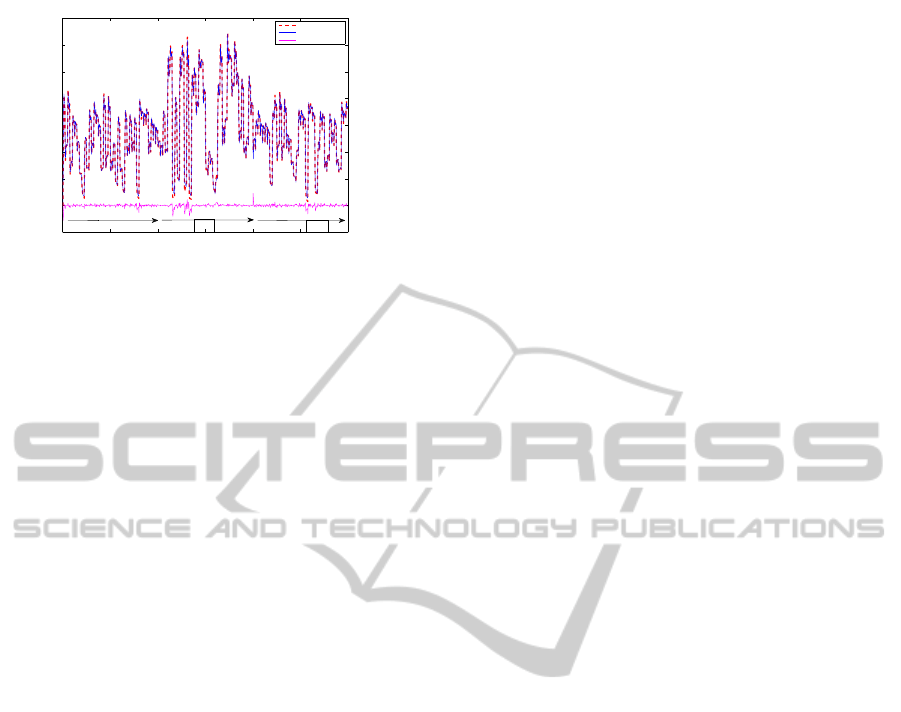
0 100 200 300 400 500 600 700 800
−1
−0.5
0
0.5
1
1.5
2
2.5
System output
Model output
Identification error
Figure 9: Identification based on LS-SVM with linear ker-
nel.
0 100 200 300 400 500 600 700 800
−1
−0.5
0
0.5
1
1.5
2
2.5
System output
Model output
Identification error
Figure 10: Identification based on LS-SVM with Gaussian
kernel.
0 100 200 300 400 500 600 700 800
−1
−0.5
0
0.5
1
1.5
2
2.5
System output
Model output
Identification error
Figure 11: Multi-kernel LS-SVM identification.
converges to 91.29% after the combination of these
two kernel functions.
Figure 11 shows that the system output and the model
output are overcome and the identification error is
acceptable. These obtained results demonstrate the
effectiveness of our provided idea in identification
problems. The same procedure is applied in the sec-
ond subsystem and the proposed multi kernel method
demonstrate once again, his performances.
The two obtained multi kernel LS-SVM model were
constructed. The global system behaviour switches
between the different models.
To evaluate identification performances obtained with
multi-model based on multi-kernel LS-SVM ap-
proach, we have considered the following sequence
”S
1
;S
2
;S
1
”. The obtained identification results are
given by the figure 12.
The considered criterion ”FIT” converges to 95.47%
ICFC 2010 - International Conference on Fuzzy Computation
314

0 200 400 600 800 1000 1200
−0.5
0
0.5
1
1.5
2
2.5
3
3.5
System output
Model output
Identification error
S2
S1
S1
Figure 12: Multi-kernel LS-SVM identification of the
global system.
which is an acceptable performance.
4 CONCLUSIONS
A multi kernel LS-SVM identification method is pro-
posed in this paper. The suggested idea consists on
training an LS-SVM algorithm with multiple kernel
functions. A linear kernel combined with the Gaus-
sian one have been chosen. These two weighted com-
bined kernels were demonstrate a good performances
in the identification context compared with the tra-
dionnal LS-SVM method which uses unique kernel
function.
REFERENCES
Bemporad, A., A. Garulli, S. P., and Vicino, A. (2005).
A bounded-error approach to piecewise affine system
identification. In IEEE Transactions on Automatic
Control, 50: 1567-1580.
Delmotte, F. (1997). Analyse multimod`ele. In Th`ese, UST
de Lille, France.
Diosan, L., Oltean, M., Rogozan, A., and Pecuchet, J.
(2007). Improving svm performance using a linear
combination of kernels. In B. Beliczynski et al. (Eds.):
ICANNGA 2007, Part II, LNCS 4432, pp. 218-227,
2007. Springer–Verlag Berlin Heidelberg 2007.
ElFerchichi, S., Laabidi, K., Zidi, S., and Maouche, S.
(2009). Feature selection using an svm learning ma-
chine. In Signals, Circuits and Systems (SCS).
Goethals, I., Pelckmans, K., Suykens, J., and Moor, B. D.
(2005). Identfication of mimo hammerstein models
using least squares support vector machines. In Sci-
ence direct, automatica 41 (2005) 1263 –1272.
Lanckriet, G. R., Cristianini, N., Bartlett, P., Ghaoui, L. E.,
and Jordan, M. (2004). Learning the kernel matrix
with semidefinite programming. In Journal of Ma-
chine Learning Research, 5, 27-72.
Lauer, F. (2008). From support vector machines to hybrid
system identification. In th`ese doctorat de l’Universit´e
Henri Poincar´e-Nancy1. sp´ecialit´e automatique.
Lei, B., Wang, W., and Li, Z. (2008). On line predictive
control based on ls svm. In Proceedings of the 7th
World Congress on Intelligent Control and Automa-
tion. Chongqing, China.
Messaoud, A., Ltaief, M., and Abdennour, R. B. (2009).
Supervision based on partial predicctors for a mul-
timodel generalised predictive control : exprimental
validation on a semi-batch reactor. In J. Modelling
Identification and control, vol 6 no 4.
Sonnenburg, S., R ¨atsch, G., Schfer, C., and Schlkopf,
B. (2006). Large scale multiple kernel learning.
In Journal of Machine Learning Research 7 (2006)
15311565.
Suykens, J. and J.Vandewalle (1999). Least squares support
vector machine classifier. In Neural Processing Let-
ters 9: 293–300,1999. Kluwer Academic Publishers.
Printed in the Netherlands.
Tao, S., Chen, D., and Zhao, W. (2009). Fast pruning al-
gorithm for multi-output ls-svm and its application in
chemical pattern classification. In Chemometrics and
Intelligent Laboratory Systems 96, 63-69.
Tarhouni, M., Laabidi, K., Zidi, S., and Ksouri, M. L.
(2010). Surveillance des systemes complexes par les
s´eparateurs `a vaste marge. In 8eme Conf´erence Inter-
nationale de MOd´elisation et SIMulation - MOSIM’10
- 10 au 12 mai 2010 - Hammamet - Tunisie.
Valyon, J. and Horvath, G. (2005). A robust ls–svm re-
gression. In Proceeding of word academy of science,
engeneering and technology, Volume 7, 148–53.
Verdult, V., Ljung, L., and Verhaegen, M. (2002). Iden-
tification of composite local linear state-space mod-
els using a projected gradient search. In International
Journal Control, 75 :1385-1398, 2002.
Zhejing, B., Daoying, P., and Youxian, S. (2004). Multi-
ple kernel learning, conic duality, and the smo algo-
rithm machine with multi–kernel. In Proceedings of
the 21
st
International Conference on Machine Learn-
ing, Banff, Canada.
Zhejing, B., Daoying, P., and Youxian, S. (2007). Nonlin-
ear model predictive control based on support vector
machine with multi–kernel. In Chin. J. Chern. Eng.,
15(5) 691–697.
Zidi, S., Maouche, S., and Hammadi, S. (2006). Nou-
velle approche pour la regulation des r´eseaux de trans-
port multimodal. 6eme Conf´erence Francophone de
MOd´elisation et SIMulation , MOSIM’06 ,du 3 au 5
avril 2006, Rabat, Maroc.
Zouari, T., Laabidi, K., and ksouri, M. (2008). Multimodel
approach applied for failures diagnostic. In Interna-
tional Journal of sciences and Techniques of Auto-
matic controle and computer engineeering, IJ–STA,
Volume 2, N1, pp. 500–515.
SYSTEM IDENTIFICATION BASED ON MULTI-KERNEL LEAST SQUARES SUPPORT VECTOR MACHINES
(MULTI-KERNEL LS-SVM)
315