NEURAL NETWORK BASED CONTROLLER FOR NONLINEAR

AUTOMATIC GENERATION CONTROL

S. Z. Rizvi, M. S. Yousuf

Department of Electrical Engineering, King Fahd Univ. of Petroleum & Minerals, Dhahran, Saudi Arabia

H. N. Al-Duwaish

Department of Electrical Engineering, King Fahd Univ. of Petroleum & Minerals, Dhahran, Saudi Arabia

Keywords:

Artiﬁcial neural network controller, Nonlinear control, Automatic generation control, Load frequency control.

Abstract:

This paper presents an Artiﬁcial Neural Network (ANN) based controller design for nonlinear multivariable

systems. The proposed method uses a novel algorithm for using and training a radial basis function (RBF)

neural network based controller. The training algorithm makes sure that it does not violate any constraints on

the inputs or outputs. Trajectory tracking results are presented for the challenging problem of nonlinear single

area Automatic Generation Control (AGC) power system. Both linear and nonlinear cases are considered and

robustness of the controller is tested as well.

1 INTRODUCTION

Artiﬁcial neural networks (ANN) have been used for

pattern recognition, function approximation, time-

series prediction and classiﬁcation problems for quite

some time (Haykin, S., 1999). Owing to their learning

capability, the use of ANN for applications requiring

intelligence, is of no surprise. Hence, like all ﬁelds,

researchers working in the ﬁeld of system theory and

control systems have been attracted to the use and de-

velopment of ANN to solve complex, nonlinear, and

often time varying real life processes. Controlling a

real life process is a task of imminent industrial sig-

niﬁcance and requires effective controller design, that

can steer the process from one operating point to an-

other, keeping in mind all the deterministic as well as

stochastic constraints and limitations on various in-

puts and outputs. The learning properties of neural

networks make them ideal for this purpose.

The use of neural network for controller design

can be found in the literature with different designs

and training techniques. Smith and Boning (Smith,

T. H., Boning, D. S., 1997) proposed a self-tuning

EWMA adaptive controller which, according to the

authors was able to replace an experienced engineer

needed to tune the controller. Thapa, Jones, and Zhu

proposed a scheme for combining back propagation

trained neural network with self tuning regulator tech-

niques (Thapa, B. K., Jones, B., Zhu, Q. M., 2000).

Other efforts to solve control problems using ANN

include, but are not limited to those of (Shukla, D.,

Dawson, D. M., Paul, F. W., 1999; Lu, J., Yahagi, T.,

2000; Hayakawa, T., Haddad, W., Hovakimyan, N.,

2000; Yang, Y., Wang, X., 2007; Hayakawa, T., Had-

dad, W., Volyanskyy, K. Y., 2008; Zayed, A. S., Hus-

sain, A., Abdullah, R. A., 2006; Petre, E., Selisteanu,

D., Sendrescu, D., 2008; Cong, S., Liang, Y., 2009),

and (Al-Duwaish, H. N., Rizvi, S. Z., 2010).

Power systems play a vital role in our lives, en-

suring proper generation, distribution, conservation,

recycling and regeneration of power for domestic as

well as commercial life. Power systems can safely be

regarded as the backbone of every industry. Hence,

proper control of power systems is an extremely im-

portant task and calls for accelerated efforts from

researchers all over the world (Shijie, Y., Xu, W.,

2009). This paper presents a new neural network

based controller design for nonlinear multivariable

systems. The design uses radial basis function (RBF)

neural network as controller. Output layer synaptic

weight are updated and weight update equations us-

ing classical least mean square (LMS) principle is de-

rived for the RBF network. Because of remarkable

adaptation properties of neural networks, the derived

322

Z. Rizvi S., S. Yousuf M. and N. Al-Duwaish H..

NEURAL NETWORK BASED CONTROLLER FOR NONLINEAR AUTOMATIC GENERATION CONTROL.

DOI: 10.5220/0003081503220329

In Proceedings of the International Conference on Fuzzy Computation and 2nd International Conference on Neural Computation (ICNC-2010), pages

322-329

ISBN: 978-989-8425-32-4

 2010 SCITEPRESS (Science and Technology Publications, Lda.)

controller is robust to accommodate parameter vari-

ations, if any, as well. The developed controller is

tested by employing it to control frequency deviation

caused by changes in loading in a power generator.

This problem is known as Load Frequency Control

(LFC) or Automatic Generation Control (AGC), and

has been an important control problem for power en-

gineers owing to its signiﬁcance in daily life.

Notations in this paper are used in the follow-

ing manner. Variables in lower case represent scalar

quantities. Lower case bold variables represent vector

quantities. Upper case bold variables represent matri-

ces. The only exceptions to this convention is in the

choice of a more conventional J for the cost function,

and where notations are deﬁned otherwise, as in the

AGC model. The paper is arranged as follows. Sec-

tion 2 takes a detailed look at the development and

training algorithm of the proposed controller. Section

3 takes a look at the power system model and deﬁnes

the AGC control problem in detail. Simulation re-

sults for the AGC problem are presented in section 4.

Finally, conclusions are drawn and recommendations

for future work are provided in section 5.

2 CONTROLLER DESIGN

Consider a multi-input multi-output nonlinear process

having p inputs and m outputs shown in Figure 1. It is

required that the process outputs follow a desired set

of reference points r(t) = [r

(t)· ··r

(t)]. The process

is approximated using a linear time-invariant (LTI)

model. This can be achieved in terms of ofﬂine sys-

tem identiﬁcation. The linearized approximation can

be expressed as

x(t + 1) = Ax(t) + Bu(t),

y(t) = Cx(t) + Du(t). (1)

The controller consists of an RBF nerual network.

The j

output of the RBF network is given by

(t) = w

(t), (2)

where w

is the vector for weights of j

RBF output,

given by

= [w

···w

], (3)

and φ(t) is the basis function vector which is given by

φ(t) = [φ(kr(t) − c

k)···φ(kr(t) − c

k)]. (4)

In the above equations, q denotes the number of neu-

rons in the hidden layer, c

is the center vector for

the i

neuron of that layer, φ is the radial basis func-

tion, and k.k denotes norm. RBF networks enjoy sev-

eral advantages over multi-layer perceptrons (MLP)s

in that RBF networks consist of only one hidden layer

as opposed to multiple layers in MLPs. Hence, the

learning time of RBF networks is much less as com-

pared to MLPs. RBF networks are also called univer-

sal approximators (Haykin, S., 1999), and hence can

approximate any continuous nonlinear function. It is

this property of RBF neural networks that has moti-

vated the authors to choose it for controller design.

RBF network can compensate for the nonlinearity in

the process, and hence can control the process using

linearized model for updating its weights.

For j = 1, 2,··· p, the constraints on any control

signal u

(t) are given by

min

≤ u

(t) ≤ u

max

To meet this constraint, the output of the RBF net-

work is transformed by a tangent-sigmoid activation

function forming the constrained control signal

(t) = α

(t)

− 1

(t)

+ 1

= α

φ(t)

− 1

φ(t)

+ 1

where α = |u

min

| = |u

max

| denotes the upper and lower

limits of the constraints and k is used to adjust the

slope of the linear part of tangent-sigmoid function.

The difference between the reference point r(t)

and the process output

y(t) gives the error e(t) =

(t)· ··e

(t)]

. In order to update the controller, a

cost function J is sought to be minimized.

J = e

(t)e(t). (5)

The RBF output layer weights are updated in the neg-

ative direction of the gradient of J. This approach,

known as the classical Least Mean Square principle is

a ‘sensible’ choice for training RBF networks accord-

ing to (Haykin, S., 1999). Hence, the weight update

equation for j

control signal u

(t) is given in equa-

tion (6) as

(k+ 1) = w

(k) − η

∂J

∂w

. (6)

Now ﬁnding the partial derivative of J w.r.t w

∂J

∂w

= 2e

(t)

∂

∂w

e(t)

= 2e

(t)

∂

∂w

(r(t) −

y(t))

= −2e

(t)

∂

∂w

y(t)

= −2e

(t)

∂

∂w

(Cx(t) + Du(t)),

NEURAL NETWORK BASED CONTROLLER FOR NONLINEAR AUTOMATIC GENERATION CONTROL

323

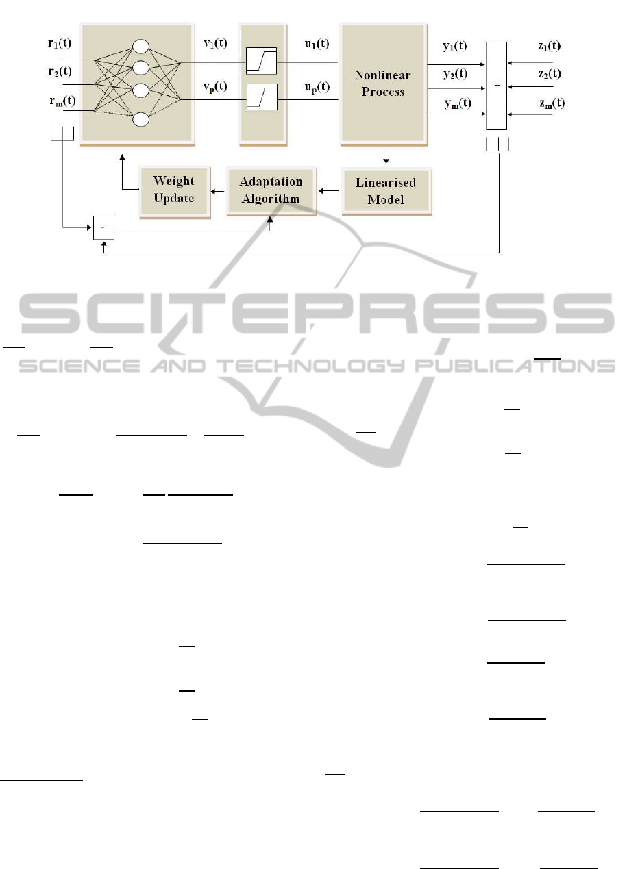
Figure 1: Neural network based controller for nonlinear MIMO systems. Parameters z

(t) indicate output additive noise at the

output.

which can be written as

∂J

∂w

= −2e

(t)

∂

∂w

(C{Ax(t − 1) + Bu(t − 1)}

+Du(t)).

The terms independent of w

would vanish,

∂J

∂w

= −2e

(t)



∂CBu(t − 1)

∂w

∂Du(t)

∂w



. (7)

Finding the derivative of tangent-sigmoid function

∂u

(t)

∂w

= α

∂

∂w

φ(t)

− 1

φ(t)

+ 1

= α

2kφ(t)e

φ(t)

+ 1)

. (8)

Equation 7 can now be written as

∂J

∂w

= −2e

(t)



CB∂u(t −1)

∂w

D∂u(t)

∂w



(9)

= −2e

(t)













·· ·ψ













∂

∂w

(t −1)

∂

∂w

(t − 1)













·· ·d













∂

∂w

(t)

∂

∂w

(t)













, (10)

Since x(t − 1) depends on u(t − 2) which in turn is a

function of w, the dependence of state vector x(t − 1) on

the weights w of the neural network is acknowledged. How-

ever the term for derivative of CAx(t − 1) w.r.t w is deliber-

ately neglected since expansion of x(t) into past state terms

Ax(t − n) + Bv(t − n) for n ≥ 2 does not yield signiﬁcant

improvement on controller result.

where Ψ ε ℜ

m×p

is the product of C ε ℜ

m×n

and B

ε ℜ

n×p

. The derivative of all terms except u

(t − 1)

and u

(t) would vanish. Substituting

∂u

(t)

∂w

from the

derivative equation 8,

∂J

∂w

= −2e

(t)













∂

∂w

(t −1)

∂

∂w

(t −1)













∂

∂w

(t)

∂

∂w

(t)













(11)

= −2e

(t)













2kφ(t−1)e

φ(t−1)

+1)

2kφ(t−1)e

φ(t−1)

+1)













2kφ(t)e

φ(t)

+1)

2kφ(t)e

φ(t)

+1)













(12)

∂J

∂w

= −2[e

(t)·· ·e

(t)] (13)







2kφ(t−1)e

φ(t−1)

+1)

+ d

2kφ(t)e

φ(t)

+1)

2kφ(t−1)e

φ(t−1)

+1)

+ d

2kφ(t)e

φ(t)

+1)







ICFC 2010 - International Conference on Fuzzy Computation

324

= 2e

(t)

2kφ(t − 1)e

φ(t−1)

+ 1)

+ d

2kφ(t)e

φ(t)

+ 1)

·· ·−2e

(t)

2kφ(t − 1)e

φ(t−1)

+ 1)

+ d

2kφ(t)e

φ(t)

+ 1)

(14)

Finally, the weight update equation for j

control

signal u

(t) becomes

(k+ 1) = w

(k) + 2η

∑

l=1

(t)

l j

2kφ(t − 1)e

φ(t−1)

+ 1)

+ d

l j

2kφ(t)e

φ(t)

+ 1)

(15)

where e

(t) corresponds to error at the l

output, ψ

l j

is the element at the l

row and j

column of the

matrix Ψ, η is the learning rate of the RBF neural

network, w

is the vector for the weights of j

RBF

output, m is the number of outputs of the process, and

φ(t) is the basis function vector.

3 THE AUTOMATIC

GENERATION CONTROL

PROBLEM

Automatic Generation Control (AGC) has been an

important subject for power engineers for quite some

time. It is also known as Load Frequency Control

(LFC) and has been under study for decades. The

problem arises from the fact that loading in power

systems is never constant, and changes in load in-

duce changes in system frequency. This is because

imbalance between real generated power and loading

causes the generator shaft speed to change, resulting

in the variation of system frequency.

Hence, a controller is needed to keep the fre-

quency of the output electrical power at the nominal

value. The input mechanical power to the generator is

used to control the load frequency. The main qual-

ity risk involved during control is that control area

frequencies can undergo prolonged ﬂuctuations due

to a sudden change of loading in an interconnected

power system as described in (Chan, W. C., Hsu, Y.

Y., 1981). These prolonged ﬂuctuations are mainly

the result of system nonlinearities. The purpose of

AGC is to track load variations and reduce these ﬂuc-

tuations. In this way, the system frequency is main-

tained, transient errors are minimized and steady state

error is avoided.

Linear and nonlinear control of AGC systems has

been studied by several researchers as in (Pan, C. T.,

Liaw, C. M., 1989; Wang, Y., Zhou, R., Wen, C.,

1993). AGC systems are modeled with nonlineari-

ties, one of the main type of which is the Generation

Rate Constraint (GRC) (Velusami, S., Chidambaram,

I. A., 2007). This is the constraint on the power

generation rate of the turbine and due to it the dis-

turbance in one area affects the output frequency in

other interconnected areas. Variable Structure Con-

trol (VSC) based techniques, (Al-Hamouz, Z. M., Al-

Duwaish, H. N., 2000), (Wang, Y., Zhou, R., Wen,

C., 1993) and Model Predictive Control (MPC) based

techniques (Yousuf, M. S., Al-Duwaish, H. N., Al-

Hamouz, Z. M., 2010), (Kong, L., Xiao, L., 2007)

have been applied to AGC and an excellent literature

survey is given in (Shayeghi, H., Shayanfar, H. A.,

Jalili, A., 2009).

3.1 AGC System Model

The block diagram of an AGC system is given in Fig-

ure 2 and the states of the system are:

X =



∆

(t)∆

(t)



. (16)

The deﬁnitions of the symbols used in the model

are as follows:

: area frequency in ith area (Hz).

: generator output for ith area (p.u. MW).

: governor valve position for ith area (p.u.

MW).

: integral control value for ith area (p.u. MW).

: tie line power output for ith area (p.u. MW).

: load disturbance for ith area (p.u. MW).

: governor time constant for ith area (s).

: plant model time constant for ith area (s).

: turbine time constant for ith area (s).

: plant transfer function gain for i

h area.

: speed regulation due to governor action for ith

area (Hz p.u. MW

−1

: frequency bias constant for ith area (p.u. MW

−1

: ratio between the base values of areas i and j.

The model can be generally represented by the fol-

lowing equations:

(t) = A

(t) + B

(t)+

∑

j=1, j6=i

(t) + F

(t), (17)

(t) = C

(t)x

(t), (18)

NEURAL NETWORK BASED CONTROLLER FOR NONLINEAR AUTOMATIC GENERATION CONTROL

325

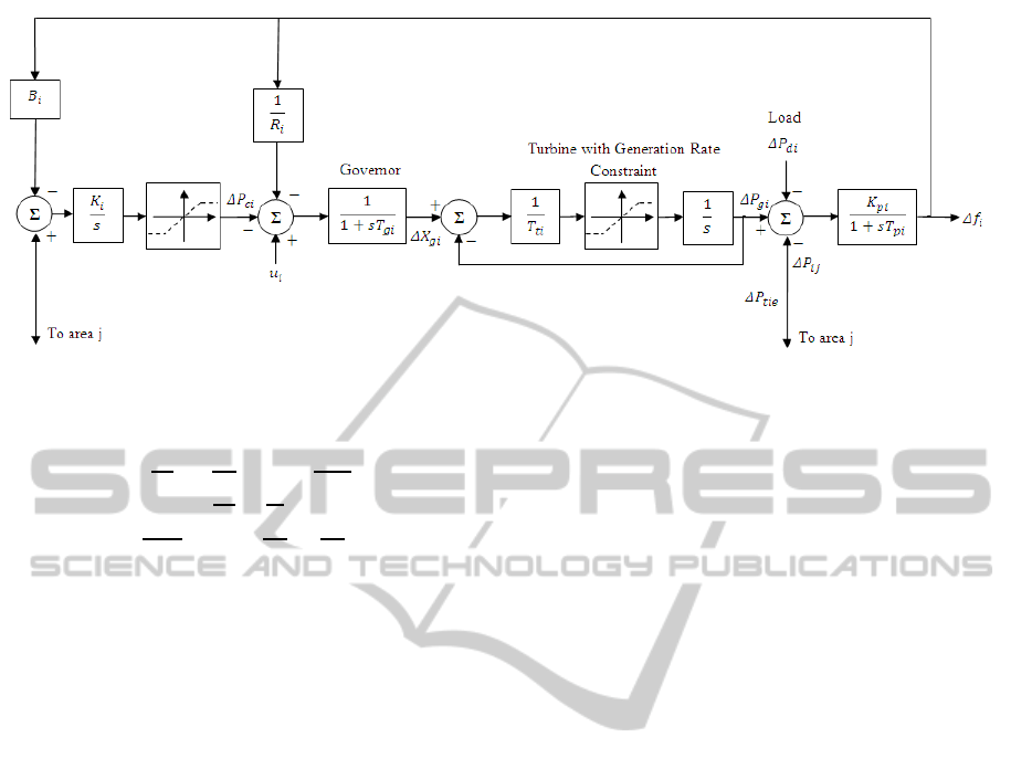
Figure 2: Block diagram of n

area AGC with GRC nonlinearities.

where







−1

−K

−1

0 0

−1

0 0 0 K

∑

0 0 0 0







,(19)

where K

is zero for single area machine.



0 0 1/T

0 0



, (20)







0 0 0 0 0

−T

0 0 0 0







, (21)



−K

0 0 0 0



, (22)

(t) = P

(t). (23)

The numerical values of these parameters are

given in Section 4. The control objective of AGC is to

keep the change in frequency, ∆ f

(t) = x

(t) as close

to 0 as possible in the presence of load disturbance,

(t) by the manipulation of the input, u

(t). The de-

tailed model of the system along with the values of

state matrices can be found in (Yang T. C., Cimen,

H., Zhu, Q. M., 1998).

3.2 Control Objective

Given a linear or nonlinear AGC system, the con-

troller objective is to construct the ANN based con-

troller such that it minimizes the error in the minimum

time using minimum effort in the presence of distur-

bances and constraints.

The disturbance is applied as a p.u. load demand.

Practically, this translates to a step load demand of a

certain percentage from the AGC system. Naturally,

this demand will cause the system to adjust its load

by the same amount to fulﬁl the quality of service.

This will change the load frequency. The proposed

controller is required to minimize this frequency de-

viation and bring it to zero in minimum time while

obeying the constraints on system states and control

signal.

4 SIMULATION RESULTS

Linear as well as the nonlinear control for a single

area AGC system is simulated. The system is sim-

ulated as a single-input single-output (SISO) system,

with one control signal being the input and frequency

deviation being the output. The cost function is given

J = e

(t)e(t)

= kr(t) −

y(t)k

where r(t) denotes reference values for frequency de-

viation, which is zero for the given control objective.

The vector

y(t) denotes the actual AGC output values

of these parameters. The AGC parameters are com-

puted using the following values:

= 20s, K

= 120 Hz p.u. MW

−1

, T

= 0.3s, T

= 0.08s, R = 2.4 Hz p.u. MW

−1

, T

= 0.05s, where

refers to discretization sampling time. The corre-

sponding values of A, B & F are:

A =







−0.05 6 0 0

0 −3.33 3.33 0

−5.208 0 −12.5 −12.5

0.6 0 0 0







, (24)

B =



0 0 12.5 0



, (25)

F =



−6 0 0 0



. (26)

ICFC 2010 - International Conference on Fuzzy Computation

326

0 5 10 15 20 25

−4

−2

x 10

−3

time(sec)

state x

reference signal

controlled output

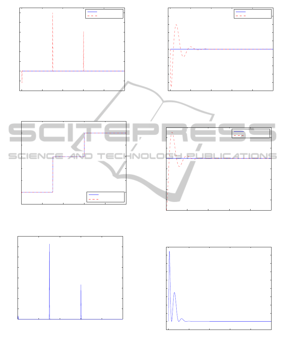
Figure 3: Frequency deviation for linear AGC.

0 5 10 15 20 25

−0.01

0.01

0.02

0.03

0.04

0.05

0.06

time(sec)

load disturbance

generated power

Figure 4: Change in generated power for linear AGC.

0 5 10 15 20 25

x 10

−5

time(sec)

mse

Figure 5: Convergence of error function for linear AGC.

While designing a controller, a suitable number of

neurons can be chosen based on experience. Repeated

simulations can then be run to test the controller with

increased number of neurons each time until no ap-

preciable increase in performance is noted. To begin

with, a network of just two RBF neurons is used for

0 5 10 15 20 25

−1

−0.8

−0.6

−0.4

−0.2

0.2

0.4

0.6

0.8

time(sec)

state x

reference signal

controlled output

Figure 6: Frequency deviation for AGC with GRC nonlinear-

ity.

0 5 10 15 20 25

0.002

0.004

0.006

0.008

0.01

0.012

0.014

0.016

time(sec)

load disturbance

generated power

Figure 7: Change in generated power for AGC with GRC non-

linearity.

0 5 10 15 20 25

−0.05

0.05

0.1

0.15

0.2

0.25

0.3

0.35

0.4

0.45

time(sec)

mse

Figure 8: Convergence of error Function for AGC with GRC

nonlinearity.

controller design. The input to the neural network is

the reference signal for frequency deviation. A neu-

ron center for each neuron is chosen around the desi-

NEURAL NETWORK BASED CONTROLLER FOR NONLINEAR AUTOMATIC GENERATION CONTROL

327

red set-point on the reference trajectory. Spread of the

gaussian basis function σ is chosen such that the RBF

functions are neither too peaked nor too ﬂat. Methods

to ﬁnd proper basis function spread exist in (Haykin,

S., 1999). A nominal spread of 0.04 is chosen. The

learning rate η has to be chosen with care as well.

Small value of learning rate can cause slow conver-

gence of error while too large a value can make the

controller unstable.

The constraint α = |u

min

| = |u

max

| on the control

signal is given by

−0.5 ≤ α ≤ 0.5.

Single area linear and nonlinear AGC is simulated

with zero initial conditions and the neural network

controller shows satisfactory control results for both

cases.

4.1 Single Area AGC excluding

Nonlinearities

First, the nonlinearity is excluded and the perfor-

mance of the proposed controller is tested for the lin-

ear system.

To study the robustness of the proposed controller,

a condition of varying load disturbance is considered.

The load is simulated to vary from a disturbance of

0 p.u. to 0.03 p.u. after 7.5 seconds, and then going

up to 0.05 p.u. after 15 seconds. This directly affects

the load frequency as seen in Figure 3. It is seen that

the load frequency varies most when the disturbance

varies most, but the neural network controller quickly

pushes it back zero. The corresponding behavior of

the change in generated power is seen in the Figure

4. It is seen that the change in generated power fol-

lows the load disturbance as well, meaning that the

system can supply the load its power demand. The

power generated changes most when the disturbance

is largest. The error convergence is given in Figure 5.

4.2 Single Area AGC including GRC

Nonlinearities

Now the case of nonlinear AGC system is considered.

The nonlinearities in the system appear in the form of

saturation on change of states x

and x

as illustrated

in Figure 2. Mathematically, the nonlinearity can be

described as

(t − 1) − GRC ≤ ∆x

(t) ≤ x

(t − 1) + GRC,

for i = 2,4

The system is tested for a practical GRC value of 0.6

p.u. MW min

−1

= 0.01 p.u. MW sec

−1

, as done

in previous work of (Wang, Y., Zhou, R., Wen, C.,

1993). This means that the generated power output of

the system cannot vary by more than 0.01 p.u. MW in

1 second. A disturbance of 1% p.u. is present in the

system. The proposed controller is applied to the sys-

tem with this nonlinearity and the results can be seen

in Figures 6, 7, and 8. The NN controller successfully

keeps the frequency deviation to zero while the Gen-

erated power follows the step change in load demand

disturbance.

5 CONCLUSIONS

A new and efﬁcient ANN based control scheme is

designed. Weight update algorithm is worked out

and the controller is shown to be viably applicable to

practical power systems. The dynamical behavior of

the single nonlinear AGC system with proposed con-

troller is examined. The proposed controller performs

well for linear as well as nonlinear case. With just

two neurons, the performance of the controller is well

acceptable under rapid load variations. Encouraging

results are a sound motivation for possible future ap-

plication of proposed controller to multiple area linear

and nonlinear AGC problem.

ACKNOWLEDGEMENTS

The authors would like to acknowledge the support

of King Fahd University of Petroleum & Minerals,

Dhahran, Saudi Arabia.

REFERENCES

Al-Duwaish, H. N., Rizvi, S. Z. (2010). Neural network

based controller for constrained multivariable sys-

tems. In 12th WSEAS Conference on Automatic Con-

trol, Modelling and Simulation ACMOS 2010, Italy,

pages 104–109.

Al-Hamouz, Z. M., Al-Duwaish, H. N. (2000). A new load

frequency variable structure controller using genetic

algorithms. In Electric Power Systems Research. vol-

ume 55, no. 1, pages 1-6.

Chan, W. C., Hsu, Y. Y. (1981). Automatic generation

control of interconnected power system using variable

structure controllers. In Proceedings of the IEE Part

C. volume 128, no. 5, pages 269-279.

Cong, S., Liang, Y. (2009). Pid-like neural network nonlin-

ear adaptive control for uncertain multivariable mo-

tion control systems. In IEEE Transaction on Indus-

trial Electronics. volume 56, no. 10, pages 288-292.

ICFC 2010 - International Conference on Fuzzy Computation

328

Hayakawa, T., Haddad, W., Hovakimyan, N. (2000). Neu-

ral network adaptive control for nonlinear uncertain

dynamical systems with asymptotic stability guaran-

tees. In IEEE American Control Conference, 2005,

USA. pages 1301-1306.

Hayakawa, T., Haddad, W., Volyanskyy, K. Y. (2008). Neu-

ral network hybrid adaptive control for nonlinear un-

certain impulsive dynamical systems. In Nonlinear

Analysis: Hybrid Systems. pages 862-874.

Haykin, S. (1999). Neural Networks - A Comprehensive

Foundation. Prentice-Hall, Second Edition.

Kong, L., Xiao, L. (2007). A new model predictive con-

trol scheme-based load-frequency control. In IEEE

International Conference on Control and Automation.

volume 1, pages 2514-2518.

Lu, J., Yahagi, T. (2000). Application of neural networks to

nonlinear adaptive control systems. In IEEE Interna-

tional Cconference on Signal Processing, ICSP, 2000.

pages 252-257.

Pan, C. T., Liaw, C. M. (1989). An adaptive controller

for power system and load frequency control. In

IEEE Transactions on Power Systems. volume 4, no.

1, pages 122-128.

Petre, E., Selisteanu, D., Sendrescu, D. (2008). Neural net-

works based adaptive control for a class of time vary-

ing nonlinear processes. In IEEE International Con-

ference on Control, Automation and Systems, ICCAS,

2008, Korea. pages 1355-1360.

Shayeghi, H., Shayanfar, H. A., Jalili, A. (2009). Load fre-

quency control strategies: A state-of-the-art survey for

the researcher. In Energy Conversion and Manage-

ment. volume 50, no. 1, pages 344-353.

Shijie, Y., Xu, W. (2009). Rbf neural network adaptive con-

trol of microturbine. In IEEE Global Congress on In-

telligent Systems. pages 288-292.

Shukla, D., Dawson, D. M., Paul, F. W. (1999). Mul-

tiple neural-network-based adaptive controller using

orthonormal activation function neural networks. In

IEEE Transaction on Neural Networks. volume 10,

no. 6, pages 1494-1501.

Smith, T. H., Boning, D. S. (1997). A self-tuning ewma

controller utilizing artiﬁcial neural network function

approximation techniques. In IEEE Transaction on

Components, Packaging, and Manufacturing Technol-

ogy, Part C. volume 20, no. 2, pages 121-132.

Thapa, B. K., Jones, B., Zhu, Q. M. (2000). Non-linear

control with neural networks. In Fourth International

Conference on knowledge-based Intelligent Engineer-

ing Sys. & Allied Tech., 2000, U.K. pages 868-873.

Velusami, S., Chidambaram, I. A. (2007). Decentralized bi-

ased dual mode controllers for load frequency control

of interconnected power systems considering gdb and

grc non-linearities. In Energy Conversion and Man-

agement.

Wang, Y., Zhou, R., Wen, C. (1993). Robust load frequency

controller design for power systems. In IEE Proceed-

ings Part C. volume 140, no. 1, pages 11-16.

Yang T. C., Cimen, H., Zhu, Q. M. (1998). Decentralised

load-frequency controller design based on structured

singular values. In IEE Proceedings on Generation,

Transmission and Distribution. volume 145, no. 1,

pages 7-14.

Yang, Y., Wang, X. (2007). Adaptive h

∞

tracking control

for a class of uncertain nonlinear systems using radial-

basis-function neural networks. In Neurocomputing.

volume 70, pages 932-941.

Yousuf, M. S., Al-Duwaish, H. N., Al-Hamouz, Z. M.

(2010). PSO based predictive nonlinear automatic

generation control. In 12th WSEAS Conference on Au-

tomatic Control, Modelling and Simulation ACMOS

2010, Italy, pages 87–92. In Press.

Zayed, A. S., Hussain, A., Abdullah, R. A. (2006). A novel

multiple-controller incorporating a radial basis func-

tion neural network based generalized learning model.

In Neurocomputing. volume 69, pages 1868-1881.

NEURAL NETWORK BASED CONTROLLER FOR NONLINEAR AUTOMATIC GENERATION CONTROL

329