
USING SLOW FEATURE ANALYSIS TO IMPROVE
THE REACTIVITY OF A HUMANOID ROBOT’S
SENSORIMOTOR GAIT PATTERN
Sebastian H
¨
ofer and Manfred Hild
Neurorobotics Research Laboratory, Computer Science Department, Humboldt-Universit
¨
at zu Berlin, Berlin, Germany
Keywords:
Slow feature analysis, Biped walking, Volterra filters, Recurrent neural networks, Sensorimotor control, Hu-
manoid robotics.
Abstract:
This paper presents an approach for increasing the reactivity of a humanoid robot’s gait, incorporating Slow
Feature Analysis (SFA), an unsupervised learning algorithm issuing from the domain of theoretical biology.
The main objective of this work is to find a means to detect disturbances in the gait pattern at an early stage
without losing stability. Another goal is to investigate the general potential of SFA for using it within sen-
sorimotor loops which to our knowledge has not been considered until now. The application of SFA within
sensorimotor loops is motivated by pointing out its relation to second-order Volterra filters. Our experiments
show that the overall reactivity of the gait pattern increases without any profound loss in stability, and that
SFA appears to be suitable for the usage even at such levels of sensorimotor control that are directly involved
into motor activity regulation.
1 INTRODUCTION
Recent trends in cognitive robotics stipulate new prin-
ciples for designing intelligent systems, amongst oth-
ers ecological balance in the complexity of the sen-
sory, motor and neural systems of the agent (Pfeifer
and Bongard, 2006). In order to develop autonomous
robots that are able to learn advanced behaviours, par-
ticularly if they are presumed to learn in a fairly un-
supervised manner, we expect the integration of re-
dundantly covered sensory data channels to be inde-
spensable for better and stable control mechanisms.
For we are dealing with real hardware and a greatly
intricate real world environment, ably integration of
high-dimensional sensory data may increase stability
and adaptivity without losing the reactivity of the dy-
namical system formed by the robot and its environ-
ment.
On the other hand, the integration of multi-
dimensional sensory data streams asks for means to
extract useful information in a computationally ef-
ficient manner. Slow Feature Analysis (SFA), the
method applied in this paper is a promising candi-
date that may fulfill the forementioned constraints and
needs.
SFA is an unsupervised learning algorithm issuing
from the domain of theoretical biology. It was develo-
ped in order to find a method for learning and extract-
ing invariances from visual data, exploiting the idea
of temporal slowness (also called temporal stability,
see e.g., (Wyss et al., 2006)), assuming that high-level
abstract features of the input signal vary slowly over
time. SFA can deal with high-dimensional data, for
it is based on the generalised eigenvalue problem, for
which fast and reliable algorithms exist. By applying
SFA to visual data, it could be shown that temporal
slowness is an important learning principle, yielding
structures that resemble cells found in the primary vi-
sual cortex and the hippocampus (Berkes and Wiskott,
2002; Franzius et al., 2007). Besides, the algorithm’s
capability to detect and extract driving forces from
non-stationary time-series (Wiskott, 2003) as well as
its use for pattern recognition (Berkes, 2006) have
been investigated.
In a recent paper, we have successfully shown
that SFA can handle many kinds of sensory qualities
by applying it to abstract visual features, accelera-
tion sensor and motor position data from humanoid
robots (Spranger et al., 2009). SFA extracted mean-
ingful components from the multisensory input data
stream, which were employed for detecting and clas-
sifying postures of humanoid robots.
In this article we demonstrate how SFA can be
used to increase the reactivity of a biped gait pattern
212
Höfer S. and Hild M..
USING SLOW FEATURE ANALYSIS TO IMPROVE THE REACTIVITY OF A HUMANOID ROBOT’S SENSORIMOTOR GAIT PATTERN.
DOI: 10.5220/0003082102120219
In Proceedings of the International Conference on Fuzzy Computation and 2nd International Conference on Neural Computation (ICNC-2010), pages
212-219
ISBN: 978-989-8425-32-4
Copyright
c
2010 SCITEPRESS (Science and Technology Publications, Lda.)

provided for a humanoid robot platform. The gait pat-
tern is neuronally implemented and based on a senso-
rimotor loop. Although the walking pattern is gen-
erally stable, robots tend to fall to the ground when
walking on surfaces with a high grip, such as carpets
or natural surfaces. Thus, a mechanism to detect when
the gait becomes unstable is needed. One of the main
problems is that the fraction of time to avoid a col-
lision with the ground or at least alleviate its effects
is very short. However, in general both high stability
and reactivity cannot be easily achieved at the same
time. We show that SFA applied to a time embedded
signal is formally equivalent to a so-called Volterra
filter, and use SFA to learn the filter weights in an un-
supervised manner. The result is a highly reactive fil-
ter, which is incorporated into the sensorimotor con-
trol loop that generates the movement, decreasing the
response time of the dynamical system formed by the
robot and its environment, and consequently provid-
ing means for a robust fall detection and prevention.
To our knowledge this is the first attempt to use
SFA components for robot control, so that the pre-
sented work also constitutes a proof of concept for
the successful application of SFA within sensorimo-
tor loops.
The remaining paragraphs will cover the follow-
ing topics: We begin with a short introduction to the
Slow Feature Analysis and Volterra filters, pointing
out why quadratic filters are a well-motivated choice
for our purposes. Next, we pass over to the experi-
ments section, presenting the robot platform that was
used for our experiments, and describe the examined
gait pattern and our modifications to it. In the last
section we present our results and show that the mod-
ifications performed prove useful for increasing the
robots reactivity without destabilisation of the gait.
We conclude this article with a summary of the ob-
tained results and by giving insights into future work.
2 METHODS
In this section we first give a brief introduction to the
Slow Feature Analysis (SFA) algorithm and its math-
ematical foundations. Then, we show that SFA yields
a solution that is formally equivalent to second-order
Volterra filters with finite kernel. In a later section, we
will exploit this relationship when we train an equiv-
alent structure by means of a supervised learning al-
gorithm and compare the obtained results.
2.1 Slow Feature Analysis
Slow Feature Analysis is an unsupervised learning
algorithm that attempts to solve a particular opti-
misation problem related to temporal slowness (see
(Wiskott, 1998) for the original publication and
(Wiskott and Sejnowski, 2002) for a more extensive
introduction). The aim of the algorithm is to extract
slowly changing features from a multi-dimensional
input signal which vary over a short time scale.
The learning problem can be stated as follows:
Given a potentially multidimensional input signal
x(t) = [x
1
, .., x
N
]
T
, N being the dimensionality of the
input, the algorithm searches for input-output func-
tions g
j
(x), j ∈ J that determine the output of the sys-
tem y
j
(t) := g
j
(x(t)). The objective function is given
as
∆(y
j
) := h ˙y
2
j
i
t
is minimal (1)
where h·i
t
signifies the average over time and ˙y is the
derivative
1
of y. The equation specifies the intended
learning problem of temporal stability, i.e., ∆(y
j
) is
minimal if y
j
varies slowly over time. However, every
constant function would easily fulfill this restriction,
so three additional constraints are formulated:
hy
j
i
t
= 0 (zero mean) (2)
hy
2
j
i
t
= 1 (unit variance) (3)
∀i < j hy
i
y
j
i
t
= 0 (decorrelation) (4)
Equation 3 forces the output signal to carry informa-
tion. Equation 4 requires the set of output functions to
be decorrelated and therefore to carry different infor-
mation and to not simply reproduce each other. It also
induces an ordering on the output signals, i.e., the first
signal y
1
will be slowest one, while the next signal y
2
will be less optimal, etc.
Since the above stated optimisation problem is
in general hard to solve, SFA provides a solution to
learning the real valued functions g
j
by simplifying
the problem: The input-output functions g
j
are con-
strained to be linear combinations of a finite set of ba-
sis functions. Let the input signal be x = [x
1
, .., x
N
]
T
,
then the input-output function g = [g
1
(x), ..., g
J
(x)]
T
can be defined as the weighted sum of K basis func-
tions h = [h
1
, .., h
k
]
T
, yielding
y
j
= g
j
(x) :=
K
∑
k=1
w
jk
h
k
(x). (5)
In the linear case no specific basis functions are
used and the input-output functions compute as the
1
The derivative is approximated by a finite difference
˙x(t) := x(t) − x(t − 1) for we are dealing with discrete sig-
nals.
USING SLOW FEATURE ANALYSIS TO IMPROVE THE REACTIVITY OF A HUMANOID ROBOT'S
SENSORIMOTOR GAIT PATTERN
213

weighted sum of the input data; this application is
called SFA(1) or linear SFA. In order to deal with
nonlinearities in the input data the basis functions are
chosen to be a polynomial, usually quadratical, ex-
pansion of the input, leaving the weight vectors w
j
to
be learnt. This technique is similar to the so-called
kernel trick (Aizerman et al., 1964), for the expanded
signal serves as a basis for the vector space of polyno-
mials or at least some finite dimensional subset of that
vector space. The unit consisting of a polynomial ex-
pansion up to degree two combined with a linear SFA
is usually referred to as SFA(2) or quadratic SFA.
Denoting the original input data or in case of
SFA(2) the expanded data, respectively by
˜
x, param-
eters are learnt by applying SFA to the mean centered
signal x =
˜
x − h
˜
xi
t
. Obviously x automatically fulfills
constraint 2. Inserting x into the objective function 1
and into equation 4 yields
∆(y
j
) = h ˙y
2
j
i
t
= w
T
j
h
˙
x
˙
x
T
i
t
w
j
=: w
T
j
Aw
j
(6)
and
hy
i
y
j
i
t
= w
T
i
hxx
T
i
t
w
T
j
=: w
T
i
Bw
j
. (7)
Furthermore, constraint 3 can be integrated into equa-
tion 1, resulting in the new objective function
∆(y
j
) =
h ˙y
2
j
i
t
hy
2
j
i
t
=
w
T
j
Aw
j
w
T
i
Bw
j
. (8)
It is known from linear algebra that the solution to
this problem is given by the generalised eigenvalue
approach:
AW = BWL, (9)
letting W = [w
1
, . . . , w
n
] be the matrix of the gen-
eralised eigenvectors and L the diagonal matrix of
the corresponding eigenvalues λ
1
, . . . , λ
n
. It can be
shown that the orthonormal set of eigenvectors sorted
in descending order accordingly to their correspond-
ing eigenvalues yields the weight vectors w
j
(Berkes,
2006).
One of the key features of the SFA algorithm is
that if the training signal shares most of the char-
acteristics of the target input signal, the learnt pa-
rameter set will generalise well on unseen data. Al-
though the previously described exact solution of the
optimisation problem is computationally demanding,
the application of a trained SFA(2) to new data sim-
ply consists in the multiplication of the nonlinearly
expanded, mean centered input signal by the SFA
weight matrix W.
Since the input signal might already be from a
high dimensional input space, SFA(2) does, due to the
polynomial expansion, heavily suffer from the curse
of dimensionality. In order to deal with the explosion
in dimensionality SFA can be applied successively
in networks of SFA modules, passing only a limited
amount of slowest components to the next module.
We will reduce the dimensionality of the input by
prepending the SFA(2) module with an SFA(1) mod-
ule.
2.2 Second-order Volterra Filters
It has been shown in (Berkes and Wiskott, 2006) that
every input-output function y
j
(t) = g
j
(x) learnt by a
quadratic SFA can be formulated in a general inho-
mogenous quadratic form as given by the following
equation:
y
j
(t) = c +f
T
x +
1
2
x
T
Hx. (10)
Letting x(t) := [x(t − m + 1), x(t − m + 2), . . . , x(t)],
i.e., a time embedded signal with tap delay m, this
form corresponds to the second-order Volterra series
with finite kernel, which provides the basis for so-
called Volterra filters, a type of well-studied nonlin-
ear FIR filters
2
(Mathews, 1991; Lau et al., 1992).
The coefficient terms c ∈ R, f ∈ R
m
and H ∈ R
m×m
are also called the filter kernels. The relation between
SFA and Volterra filters is interesting insofar as clas-
sic approaches for the design of these filters focus on
supervised adaptation, whereas the SFA is a strictly
unsupervised method.
In fact, quadratic filters are very suitable for the
use with dynamic acceleration sensory data: As de-
scribed in the next section, the robot platform used in
this paper features several pairs of orthogonal acceler-
ation sensors. The two-dimensional vector x formed
by the values of an orthogonal acceleration sensor pair
can be expressed by polar coordinates,
x
1
= r cos(φ), x
2
= r sin(φ), (11)
and obviously, the squared sum of the two sensors
eliminates the sinus and cosinus terms,
x
2
1
+ x
2
2
= r
2
, (12)
thus, being proportional to the energy. As shown be-
low, the described filter learning algorithms exploit
this fact in order to separate the sensory input signal
into dynamic and static parts, facilitating the smooth-
ing of the signal.
3 EXPERIMENTS
Our experiments were conducted on a humanoid
robot platform which was developed at our laboratory
2
Finite impulse response filters.
ICFC 2010 - International Conference on Fuzzy Computation
214

Figure 1: Extract from a high speed video depicting the movement in the coronal plane.
specifically for researching basic motion capacities,
most importantly biped walking. In this section we
briefly describe our robot platform, the examined gait
pattern and how we use SFA for our aim of increasing
its reactivity.
3.1 Embodiment
The humanoid robots used in our experiment are
robots of the so-called A-series platform. The robot
is based on a commercially available robot kit, called
Bioloid, which was augmented by additional process-
ing power, a camera in the head and several proprio-
ceptive sensors. The robot features 21 degrees of free-
dom, 19 in the body, including elbow, hand, hip, knee
and foot joints, as well as motors driving the pan-and-
tilt unit for the camera. Eight microprocessor boards
are distributed across the body for actuator control,
additionally featuring a two-axes acceleration sensor
each. The boards are located on the hips, arms and
shoulders. Each board controls up to two actuators,
while communicating via a shared system bus, that in-
tegrates incoming and outgoing data from the sensors
and the motors. Throughout our experiments all sen-
sory and motor values were normalised to [−1.0, 1.0].
3.2 Gait Pattern
The studied gait pattern is based on a neurally imple-
mented sensorimotor loop, which was developed at
our laboratory. The underlying neural model consists
of standard time discrete units using the hyperbolic
tangent as a nonlinear transfer function.
The gait pattern starts with an oscillation in the
coronal plane, initiated by letting the robot move its
feet such that it subsequently displaces its weight
from one foot to the other in order to get the feet off
the ground. Figure 1 shows a series of snapshots from
a high speed video depicting this coronal movement.
Then, as soon as a sensory threshold is reached, the
robot starts moving its feet to the front, beginning to
walk.
In this article we concentrate on a specific piece
of the whole network, namely the part responsible for
the creation of the oscillating movement in the coro-
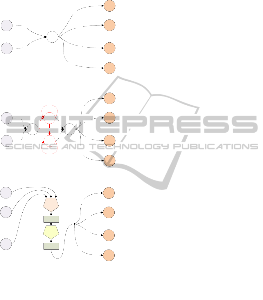
nal plane. Figure 2 shows the corresponding neu-
ral networks. The blue circles indicate input coming
from the robot’s sensors, red circles output to the mo-
tors and finally white circles represent the foremen-
tioned neural units. A possible bias value is written
into the neuron. The input values received by the net-
work consist of data from two acceleration sensors
that are located on the robot’s left and right shoulder
and direct to the coronal plane. The calculated out-
put value is passed to the robot’s hip and ankle roll
motors.
In figure 2(a), the first version of the gait net-
work is depicted, which will be called the unfiltered
gait network. The inputs are fed into a neuron where
they are equally weighted, summed and possibly dis-
torted by the nonlinearity of the hyperbolic tangent.
In this version of the network the output of the neuron
is immediately fed into the motor outputs; however,
conducting the unfiltered signal directly to the motors
results in high energy consumption and a less stable
movement pattern because of high frequency compo-
nents, which are contained in the possibly noisy ac-
celeration sensor data. Therefore, as shown in figure
2(b), two IIR filters
3
in terms of two leaky integrators
connected in parallel (red neurons and weights) were
introduced into the network serving as a low-pass fil-
ter. We will call this network the IIR gait network.
3.3 Training Data
In order to use the SFA(2) module within the senso-
rimotor loop, the module has to be passively trained
on a recorded walking sequence. For comparison, dif-
ferent sequences were generated and used as training
data: The first type of sequences was generated us-
ing the unfiltered gait network, the second type using
the IIR gait network. The sequences consisted only
of the walking pattern and did mostly not contain any
remarkable disturbances. Sequences were recorded at
100 Hz and were up to 60 seconds long.
In each case the slowest component was used for
the motor outputs. However, the slowest component
had to be multiplied by −0.1 since the sign switched
according to the coronal acceleration sensor, and it
also had to be rescaled in order to be used as a motor
control value.
3
Infinite impulse response filters.
USING SLOW FEATURE ANALYSIS TO IMPROVE THE REACTIVITY OF A HUMANOID ROBOT'S
SENSORIMOTOR GAIT PATTERN
215
0.03
-0.03
0.3
0.18
0.18
0.3
SLy_fr
SRy_fr
LHipRoll
LAnkleRoll
RHipRoll
RAnkleRoll
0.5
0.5
(a) Without Filter.
0.03
-0.03
0.3
0.18
0.18
0.3
SLy_fr
SRy_fr
LHipRoll
LAnkleRoll
RHipRoll
RAnkleRoll
0.5
0.5
0.08
0.088
-1.1
0.8
0.92
0.92
(b) With IIR Filter.
0.03
-0.03
0.3
0.18
0.18
0.3
SLy_fr
FLx_fr
LHipRoll
LAnkleRoll
RHipRoll
RAnkleRoll
Expansion
Time
Embedding
SFA
SFA
0.1
SLx_sa
.
.
.
(c) With SFA Filter.
Figure 2: Sensorimotor loops generating an oscillation in
the coronal plane. Top: Raw sensorimotor loop without any
filter. Middle: Intermediate smoothing with an IIR filter
(red structure). SLy fr and SRy fr denote the robot’s coro-
nal shoulder acceleration sensors. Bottom: Replacing the
IIR filter by an SFA module. Integrating more sensors into
the SFA module yields more stable output components.
3.4 Application of the SFA
An obvious drawback of using a leaky integrator to
filter the sensory input is that it decreases the reactiv-
ity of the whole network. Therefore, the filter structu-
re was replaced by an SFA module as depicted in fig-
ure 2(c). In contrast to the IIR filter more accelera-
tion sensor values were integrated, namely four sen-
sors from both shoulders and another four sensors lo-
cated at the robot’s feet (overall four sensors directing
to the coronal plane and four to the sagittal plane).
All 16 sensors could have been used, but in order to
keep computational cost low the number of sensors
was reduced as long as no deterioration of the result-
ing SFA(2) components was observed. Interestingly,
the resulting components were slightly better when
also sagittal sensors were fed into the SFA(2) mod-
ule. As previously mentioned, this is owed to the fact
that the orthogonal sensor pairs facilitate the extrac-
tion of dynamic components.
The employed SFA module consists of several
subunits: First, the incoming sensory data is embed-
ded in time. The number of tap delays was set to
m = 8, i.e., the current and the seven prior sensory
data values were passed to the SFA unit, which was
empirically evaluated to be a good compromise be-
tween computational effort and smoothness of the re-
sulting signal. In the next step, the result from the
time embedding is fed into a linear SFA unit which
reduces the dimensionality of the signal to 16 com-
ponents. Then the 16 components are expanded us-
ing a polynomial expansion up to degree 2 and at
last passed to a final SFA unit, together forming an
SFA(2) unit. Output signals from both the linear
and the quadratic SFA units are cut off and bound to
[−10.0, 10.0] in order to prevent from very high val-
ues caused by the polynomial expansion. Only the
first and thus slowest component y
1
of the final SFA
unit is considered and used as a driving force for the
motor outputs.
Although we described in (Spranger et al., 2009)
that it is possible to obtain very smooth resulting SFA
components by the application of several subsequent
SFA steps and without time embedding, this method
is inappropriate for this task. The reason is that a
cascade of subsequent SFA components adapts very
strongly to the training data, causing heavily jittered
components if applied to even slightly differing un-
seen input data.
4 RESULTS
We conducted several experiments with our robots,
using the SFA implementation available from the
open source Modular Toolkit for Data Processing
(MDP) (Zito et al., 2009).
In order to compare the obtained signals the η
value proposed in (Wiskott and Sejnowski, 2002) was
ICFC 2010 - International Conference on Fuzzy Computation
216

used:
η(y) :=
T
2π
p
∆(y), (13)
a smaller value indicating slower signals.
4.1 Extracted SFA Components
Figure 3 plots data stemming from an extract of an
SFA training sequence generated by the unfiltered gait
network. The acceleration sensor data mix, the sig-
nal obtained by the application of the IIR filter to the
acceleration data mix and the slowest component ex-
tracted by the SFA module are depicted. All signals
were whitened before plotting for better comparabil-
ity and calculation of η values. The acceleration data
mix’s η value being at 10.45 is much higher than the
values of the IIR and SFA filtered signals ranging both
at about 2.9. It is obvious that the resulting slowest
component is highly correlated to both the accelera-
tion data mix and to the IIR filtered signal. However,
a short delay in the SFA module compared to the other
signals issuing from the time delay is observable. As
shown later this has no negative impact on the reactiv-
ity of the system, although it does slightly lower the
maximum frequency of the coronal oscillation. The
SFA components resulting from training on a IIR gait
network looked similar.
4.2 Comparison to an LMS Adaptive
Volterra Filter
As mentioned before, the trained SFA module corre-
sponds to a second-order Volterra filter. Therefore,
we compared the SFA module to a filter obtained
by an adaptive algorithm based on a straightforward
least mean squares (LMS) approach (Lau et al., 1992),
(Zaknich, 2005, chapter 10.4). The algorithm was
trained with the input data and the same tap delay
as the SFA (m = 8), the IIR filter output was used
as the supervisor signal. The weight terms were ini-
tialised with small random values and different learn-
ing rates µ were tested. Applied to the same acceler-
ation data mix as depicted in figure 3, the optimal re-
sult of η = 4.36 was achieved with µ = 0.01, yielding
a slightly worse result than the SFA and IIR filters.
The examination of the weights learnt by the
Volterra filter as well as the SFA component shows,
that both learning algorithms combine the linear and
the quadratic part in an identical manner: The lin-
ear part contains the main oscillation of the signal,
whilst the quadratic part is irrespective of the oscilla-
tory movement and only captures high-frequent com-
ponents. Hence, by means of the quadratic part high-
frequent and noisy components can be removed from
the signal. Figure 4 shows the slowest SFA compo-
nent and its quadratic and linear parts.
4.3 Using SFA in the Sensorimotor
Loop
As the slowness criterion is not equivalent to the def-
inition of an ideal low-pass filter, it is by no means
guaranteed that the trained SFA module repels high
frequencies, and therefore there is a risk that high-
frequency components become predominant in the
signal and lead to instability of the whole gait. Any-
way, the SFA module built into the network structure
provided a stable walking gait when trained on walk-
ing sequences generated by the unfiltered gait net-
work. Unforeseen motor activity with strong jitters
was only experienced if the robot was not upright but
laid down or the like; obviously, this jitters can eas-
ily be avoided, e.g., by using an SFA posture detector
signal inhibiting motor activity in non-upright posi-
tions.
Surprisingly, using an SFA module trained on se-
quences stemming from the IIR gait network yielded a
less stable gait and provoked more jitters. We hypoth-
esise that training an SFA module with noisier input
makes the resulting module more sensitive to the ex-
perienced noise and therefore more stable.
Table 1 summarises the properties of the different
gait networks. For each of the presented networks,
a sequence of 40 seconds was recorded. In order to
obtain the average frequency of the frontal oscillatory
movement of the resulting gait, the autocorrelation of
the equally weighted sum of the two frontal shoul-
der acceleration sensors was calculated. While the
unfiltered gait network and the IIR filtered gait net-
work produce an oscillation with almost the same fre-
quency, the SFA gait network produces a less dynamic
movement due to the aforementioned tap delay. The
increased amplitude of the unfiltered gait net results
from instabilities during the training sequence.
Table 1: The average frequency and its amplitude for the
oscillatory movement resulting from the different gait net-
works.
Frequency (Hz) Amplitude
No filter 0.01475 0.41
IIR 0.01525 0.33
SFA 0.01275 0.32
USING SLOW FEATURE ANALYSIS TO IMPROVE THE REACTIVITY OF A HUMANOID ROBOT'S
SENSORIMOTOR GAIT PATTERN
217
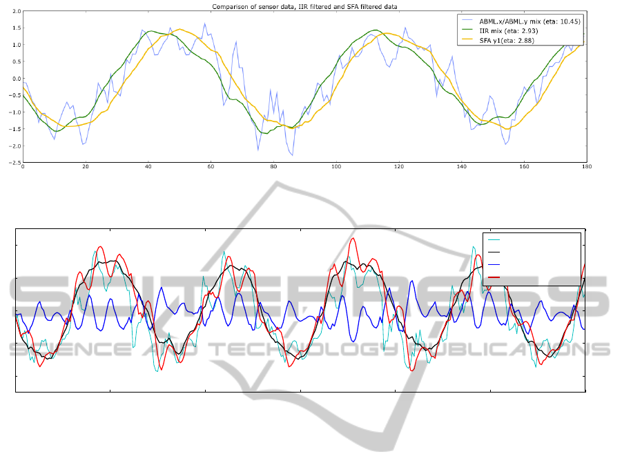
Figure 3: Comparing a weighted sum of the coronal acceleration sensors located at the shoulders to an IIR filtered signal and
the slowest component extracted by SFA.
0 50 100 150 200 250 300
−2
−1
0
1
2
SLy_fr
y
1
y
1
quadratic part
y
1
linear part
Figure 4: The slowest SFA component, separated into its linear and its quadratic part. The linear part contains the oscillatory
movement while the quadratic part consists of noisy
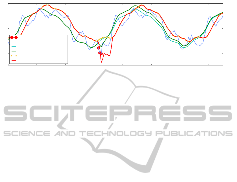
4.4 Impact of Disturbances
Now that we have shown the stability of the modified
gait network using SFA, we have to give evidence that
the reactivity of the system increases. In order to do
so we consider an artificially disturbed input signal
and compare the response of the trained SFA mod-
ule to the response of the IIR filter. Figure 5 shows
both reactions to an artificial stimulus, consisting of
an increasing negative value of 3 time steps (30 mil-
liseconds) duration added to all coronal sensors. The
dotted lines indicate how the IIR filter or the SFA
module, respectively, react on the non-disturbed sig-
nal, the continuous lines show the reaction to the dis-
turbance which is indicated by the red dots. While
the IIR filter remains almost unchanged, the distur-
bance exhibits strong impact on the SFA component
immediately. When disturbing the acceleration sen-
sors with positive values, the SFA component also ex-
hibits a remarkable reaction.
5 CONCLUSIONS AND FUTURE
WORK
We have demonstrated how Slow Feature Analysis, an
unsupervised learning algorithm based on the slow-
ness principle can successfully be integrated into sen-
sorimotor loops for advanced robot control. Using
a time embedded signal of noisy acceleration sensor
data recorded during a walk sequence of a humanoid
robot as training data for the SFA, we get a structure
that is formally equivalent to a second-order Volterra
filter. The obtained filter structure extracts the gait
pattern’s main characteristics from the training data
in a reliable and unsupervised manner, reducing noise
and disturbances. More importantly, the filter can be
used within the sensorimotor loop for the generation
of the walking pattern and its characteristics exhibit
higher reactivity than a comparable IIR filter.
This insight reveals new perspectives for the op-
portunities to use SFA for signal processing and
within sensorimotor loops, even at low levels which
are directly involved in motor activity control.
Equally, the new structure allows faster detection
ICFC 2010 - International Conference on Fuzzy Computation
218
300 320 340 360 380 400 420 440
−2
−1
0
1
2
IIR vs. SFA: Simulated short-term disturbances
Simulated disturbance
SLx_fr/SRx_fr mix
IIR filter mix
IIR filter mix with disturbance
SFA y
1
SFA y
1
with disturbance
Figure 5: Comparing the response to a short disturbance of the IIR filtered signal and the slowest component extracted by
SFA.
of undesirable configurations of the robot.
Future work will focus on how the achieved in-
crease in reactivity can be efficiently used for the im-
provement of the safety of the gait pattern. Several ap-
proaches are conceivable, e.g., the reduction of motor
activity as soon as the SFA signal leaves its allowed
range. Also one could imagine to use predictors that
are trained on the SFA component; a high prediction
error would then indicate upcoming problems.
Another promising investigation is the online
adaption of the calculated SFA component by an
adaptive LMS algorithm as mentioned in 4.2. This
would prove helpful in cases when the robot’s sensors
are exchanged and therefore slight decalibration may
occur.
In addition, further investigation will be carried
out on the applicability of SFA to other use cases for
humanoid robotics. The newly available successor of
the A-series platform, the Myon robot, is equipped
with a higher amount and additional modalities of
sensors, like pressure sensors located in the feet, etc.
Considering the results hitherto, SFA can prove useful
for the extraction of robust high level abstract features
that meaningfully describe the robot’s states on one
hand, and stabilise robot control on the other hand.
ACKNOWLEDGEMENTS
This work has been supported by the European re-
search project ALEAR (FP7, ICT-214856).
REFERENCES
Aizerman, A., Braverman, E. M., and Rozoner, L. I.
(1964). Theoretical foundations of the potential func-
tion method in pattern recognition learning. Automa-
tion and Remote Control, 25:821–837.
Berkes, P. (2006). Temporal slowness as an unsupervised
learning principle. PhD thesis, Humboldt-Universit
¨
at
zu Berlin.
Berkes, P. and Wiskott, L. (2002). Applying Slow Feature
Analysis to Image Sequences Yields a Rich Reper-
toire of Complex Cell Properties. In Dorronsoro,
J. R., editor, Proc. Intl. Conf. on Artificial Neural Net-
works - ICANN’02, Lecture Notes in Computer Sci-
ence, pages 81–86. Springer.
Berkes, P. and Wiskott, L. (2006). On the analysis and inter-
pretation of inhomogeneous quadratic forms as recep-
tive fields. Neural Computation, 18(8):1868–1895.
Franzius, M., Sprekeler, H., and Wiskott, L. (2007). Slow-
ness and sparseness lead to place, head-direction,
and spatial-view cells. PLoS Computational Biology,
3(8):e166.
Lau, S., Leung, S., and Chan, B. (1992). A reduced rank
second-order adaptive volterra filter. In ISSPA 92, Sig-
nal Processing and its Applications, pages 561–563,
Gold Coast, Australia.
Mathews, J. (1991). Adaptive polynomial filters. IEEE Sig-
nal Processing Magazine, 8(3):10–26.
Pfeifer, R. and Bongard, J. C. (2006). How the Body Shapes
the Way We Think: A New View of Intelligence (Brad-
ford Books). The MIT Press.
Spranger, M., H
¨
ofer, S., and Hild, M. (2009). Biologically
inspired posture recognition and posture change de-
tection for humanoid robots. In Proc. IEEE Interna-
tional Conference on Robotics and Biomimetics (RO-
BIO), pages 562–567, Guilin, China.
Wiskott, L. (1998). Learning Invariance Manifolds. In Proc.
of the 5th Joint Symp. on Neural Computation, May
16, San Diego, CA, volume 8, pages 196–203, San
Diego, CA. Univ. of California.
Wiskott, L. (2003). Estimating Driving Forces of Nonsta-
tionary Time Series with Slow Feature Analysis.
Wiskott, L. and Sejnowski, T. (2002). Slow Feature Anal-
ysis: Unsupervised Learning of Invariances. Neural
Computation, 14(4):715–770.
Wyss, R., K
¨
onig, P., and Verschure, P. F. M. J. (2006). A
model of the ventral visual system based on temporal
stability and local memory. PLoS Biol, 4(5).
Zaknich, A. (2005). Principles of adaptive filters and self-
learning systems. Springer London.
Zito, T., Wilbert, N., Wiskott, L., and Berkes, P. (2009).
Modular toolkit for Data Processing (MDP): a Python
data processing frame work.
USING SLOW FEATURE ANALYSIS TO IMPROVE THE REACTIVITY OF A HUMANOID ROBOT'S
SENSORIMOTOR GAIT PATTERN
219
