
SMART GROWING CELLS
Hendrik Annuth and Christian-A. Bohn
Computer Graphics & Virtual Reality, Wedel University of Applied Sciences, Feldstr. 143, Wedel, FR, Germany
Keywords:
Neural networks, Unsupervised learning, Self-organization, Growing cells structures, Surface reconstruction.
Abstract:
General unsupervised learning or self-organization places n-dimensional reference vectors in order to match
the distribution of samples in an n-dimensional vector space. Beside this abstract view on self-organization
there are many applications where training — focused on the sample distribution only — does not lead to a
satisfactory match between reference cells and samples.
Kohonen’s self-organizing map, for example, overcomes pure unsupervised learning by augmenting an addi-
tional 2D topology. And although pure unsupervised learning is restricted therewith, the result is valuable in
applications where an additional 2D structure hidden in the sample distribution should be recognized.
In this work, we generalize this idea of application-focused trimming of ideal, unsupervised learning and
reinforce it through the application of surface reconstruction from 3D point samples. Our approach is based
on Fritzke’s growing cells structures (GCS) (Fritzke, 1993) which we extend to the smart growing cells (SGC)
by grafting cells by a higher-level intelligence beyond the classical distribution matching capabilities.
Surface reconstruction with smart growing cells outperforms most neural network based approaches and it
achieves several advantages compared to classical reconstruction methods.
1 INTRODUCTION
The idea of developing the smart growing cells ap-
proach is driven by the need for an algorithm for
robust surface reconstruction from 3D point sample
clouds.
The demand for efficient high quality reconstruc-
tion algorithms has grown significantly in the last
decade, since the usage of 3D point scans has widely
been spread into new application areas. These in-
clude geometric modeling to supplement interactive
creation of virtual scenes, registering landscapes for
navigation devices, tracking of persons or objects in
virtual reality applications, medicine, or reverse engi-
neering.
3D points, retrieved by laser scanners or stereo
cameras, introduce two vital questions. First, how
can one recognize a topology of the originating 2D
surfaces just from independent 3D sample points and
without any other information from the sampled ob-
jects? Second, for further processing, how is it pos-
sible to project this topological information on a data
structure like a triangle mesh — meeting given con-
straints concerning mesh quality and size?
Although this issue has intensely been tackled
since the early eighties (Boissonnat, 1984) a general
concept that addresses all the problems of surface
reconstruction has not been determined up to now.
Noise contained in the sample data, anisotropic point
densities, holes and discontinuities like edges, and fi-
nally, handling vast amounts of sampling data with
adequate computing resources are still a big chal-
lenge.
Previous Work. The issue of surface reconstruc-
tion is a major field in computer graphics. There are
numerous approaches with different algorithmic con-
cepts. In (Hoppe et al., 1992) and (Hoppe, 2008) an
implicit surface is created from point clouds which
then is triangulated by the marching cubes approach.
(Edelsbrunner and Mcke, 1994) and (Kolluri et al.,
2004) reduce a delaunay tetrahedralization of a point
cloud until the model is carved out. Approaches like
(Storvik, 1996) or (Huang et al., 2007) utilize tech-
niques based on the Bayes’ theorem.
In the area of artificial neural networks a famous
work is (Kohonen, 1982). They propose the Self Or-
ganizing Map (SOM) which iteratively adapts its in-
ternal structure — a 2D mesh — to the distribution of
a set of samples and enables clustering or dimension-
ality reduction of the sample data. While a SOM has
a fixed topology, the growing cells structures concept
227
Annuth H. and Bohn C..
SMART GROWING CELLS.
DOI: 10.5220/0003085202270237
In Proceedings of the International Conference on Fuzzy Computation and 2nd International Conference on Neural Computation (ICNC-2010), pages
227-237
ISBN: 978-989-8425-32-4
Copyright
c
2010 SCITEPRESS (Science and Technology Publications, Lda.)

(Fritzke, 1993; Fritzke, 1995) allows the network for
dynamically fitting its size to the sample data com-
plexity. SOM and GCS are suitable for processing
and representing vector data like point samples on
surfaces. (Hoffmann and Vrady, 1998) uses a SOM
and (Vrady et al., 1999) and (Yu, 1999) a GCS for the
purpose of surface reconstruction. Further improve-
ments are made by (Ivrissimtzis et al., 2003b) where
constant Laplacian smoothing (Taubin, 1995) of sur-
faces is introduced, and in (Ivrissimtzis et al., 2003a)
the curvature described by the input sample distribu-
tion is taken to control mesh density. In (Ivrissimtzis
et al., 2004a) the GCS reconstruction process is fur-
ther enhanced in order to account for more complex
topologies. (Ivrissimtzis et al., 2004b) use several
meshes of the same model for a mesh optimization
process, and (Yoon et al., 2007) present a concept for
combining common deterministic approaches and the
advantages of the GCS approach.
Overview. In the following, we outline the basis of
our approach — the growing cells structures — and
then derive our idea of the smart growing cells, which
matches the specific requirements of reconstruction.
Afterwards, an analysis is compiled discussing mesh
quality and performance of our approach, and finally,
we close with a summary and a list of future options
of this work.
2 RECONSTRUCTION WITH
SMART GROWING CELLS
Classical growing cells approaches for reconstruction
tasks are based on using the internal structure of the
network as a triangulation of the object described by a
set of surface sample points. A 2D GCS with 3D cells
is trained by 3D points. Finally, the cells lie on the
object surface which the 3D points represent and the
network structure — a set of 2D simplices (triangles)
— is directly taken as triangulation of the underlying
3D object.
The reason for using a GCS scheme for recon-
struction tasks are its obvious advantages compared
to deterministic approaches.
• They can robustly handle arbitrary sample set
sizes and distributions which is important in case
of billions of unstructured points.
• They are capable of reducing noise and ply dis-
continuities in the input data.
• They are capable of adaption — it is not required
to regard all points of the sample set on the whole.
Further, incrementally retrieved samples can be
used to retrain the network without starting the tri-
angulation process from scratch.
• They guarantee to theoretically find the best solu-
tion possible. Thus, approximation accuracy and
mesh quality are automatically maximized.
Nevertheless, these advantages partly clash with the
application of reconstruction. On the one hand, dis-
continuities are often desired (for example, in case of
edges or very small structures on object surfaces). On
the other hand, smoothing often destroys important
aspects of the model under consideration (for exam-
ple, if holes are patched, if separate parts of the un-
derlying objects melt into one object, or if the object
has a very complex, detailed structure). In such cases,
GCS tend to generalize which may be advantageous
from the physical point of view, but which mostly lets
vanish visually important features which the human is
quite sensitized to.
The presented smart growing cells approach ac-
counts for these application-focused issues and em-
phasizes that modification of the general learning task
in the classical GCS is suitable for many novel appli-
cation fields.
2.1 Unsupervised Learning and
Growing Cells Structures
General unsupervised learning is very similar to k-
means clustering (MacQueen, 1967) which is ca-
pable of placing k n-dimensional reference vectors
in a set of n-dimensional input samples such that
they are means of those samples which lie in the n-
dimensional Voronoi volume of the reference vectors.
Adaption of reference vectors is accomplished by
randomly presenting single n-dimensional samples
from the input sample set to the set of n-dimensional
reference vectors and moving them in n-dimensional
space, described as follows.
Place k reference vectors c
i
∈ R
n
, i ∈ {0..k −
1} randomly in nD space of input samples.
repeat
Chose sample s
j
∈ R
n
randomly from the
input set.
Determine reference vector c
b
(best
matching or winning unit) closest to s
j
.
Move c
b
in the direction of s
j
according to
a certain strength ε
bm
, like c
new
b
= c
old
b
(1 −
ε
bm
) + s
j
· ε
bm
.
Decrease ε
bm
.
until ε
bm
≤ certain threshold ε
0
.
ICFC 2010 - International Conference on Fuzzy Computation
228

Surface reconstruction with pure unsupervised
learning would place a set of reference vectors on
object surfaces, but does not determine information
about the underlying surface topology. This leads to
the Kohonen Self Organizing Map.
Kohonen Self Organizing Map. The SOM is
based on reference vectors which now are connected
as a regular 2D mesh. The learning rule is extended to
account for the direct neighborhood of a best match-
ing unit as follows.
for all c
nb
∈ neigborhood of c
b
do
Move c
nb
in the direction of s
j
accord-
ing to a certain strength ε
nb
, like c
new
nb
=
c
old
nb
(1 − ε
nb
) + s
j
· ε
nb
.
Decrease ε
nb
.
end for
Insertion of this neighborhood loop into the general
unsupervised learning algorithm (after moving of c
b
)
leads to the phenomenon that the reference vertices
now are moved by accounting for the regular 2D mesh
topology of the SOM. Training a plane-like sample
set leads to an adaption of the SOM grid to this im-
plicit plane — the sample topology is recognized and
finally represented by the SOM mesh.
Nevertheless, the mesh size of a SOM is fixed
and cannot adjust to the sample structure complexity.
The growing cells structures approach overcomes this
drawback.
Growing Cells Structures. To a certain degree,
GCS may be seen as SOM which additionally are ca-
pable of growing and shrinking according to the prob-
lem under consideration which is defined by the sam-
ple distribution. This mechanism is based on a so
called resource term contained in every reference vec-
tor and which — in the original approach — is a sim-
ple counter. It counts the reference vector being a best
matching unit. A high counter value signalizes the re-
quirement for insertion of new reference vectors.
With a GCS we could train a sample set lying
on a certain object surface and the network structure
would fit the object surface at a certain approxima-
tion error. The problem is that in reconstruction tasks
sample distributions are often not uniform. The rep-
resented surfaces usually contain discontinuities like
sharp edges and holes, and the objects to be recon-
structed are not that simple like a plane or a tetrahe-
dron — which usually are chosen as initial network
and which can hardly adapt to complex topologies.
Only objects which are homeomorphic to the start ob-
ject can be represented satisfactorily.
Thus, general unsupervised learning should
evolve to a kind of constrained unsupervised learning
which detects and adapts to certain structures which
the sample set implicitly contains.
2.2 Smart Growing Cells
Smart growing cells are an application-focused, six-
way adaption of the general learning scheme of the
classical growing cells structures approach. The SGC
basic structure is identical to general GCS. There are
n-dimensional cells which we now term neural ver-
tices connected by links through an m-dimensional
topology.
We let n = 3 since neural vertices are directly
taken as vertices of the triangulation mesh and m = 2
since we aim at 2D surfaces to be reconstructed.
The main training loop is outlined in Fig. 1. Here
k
del
and k
ins
are simple counter parameters defined
below (see section 2.3). Movements of vertices and
their neighbors slightly differ from the classical SOM.
Again, there are two parameters for the learning rates,
ε
bm
for the winner and ε
nb
for its neighbors, but these
are not decreased during learning since vertex con-
repeat
for j = 1 to k
del
do
for i = 1 to k
ins
do
Choose sample s from point cloud ran-
domly, find closest neural vertex and
move it together with neighbor ver-
tices towards s.
Increase signal counter at s (the re-
source term mentioned above) and de-
crease the signal counters of all other
vertices.
end for
Find best performing neural vertex (with
highest signal counter value) and add
new vertex at this position (see Fig. 2).
end for
Find worst performing neural vertices,
delete them and collapse regarding edges
(see Fig. 2).
until certain limit like approximation error, or
number of vertices is reached.
Figure 1: Classical growing cells structures algorithm.
SMART GROWING CELLS
229

Figure 2: Neural vertex split operation (from left to right) to
increase mesh granularity locally, and edge collapse (from
right to left) to shrink mesh locally.
nections automatically become smaller together with
the learning rates. For drawing the neighboring ver-
tices, a smoothing process like described in (Ivris-
simtzis et al., 2003b) and (Taubin, 1995) is applied,
which replaces the classical movement, and which
makes the adaption of the topology more robust.
As initial network, usually a tetrahedron or a plane
with random vertices is suitable.
Vertex Split. A neural vertex split operation adds
three edges, two faces, and a new neural vertex. The
longest edge at the neural vertex with the highest re-
source term is split and a new vertex is added in the
middle. The signal counter value is equally spread
between the two vertices (see Fig. 2).
Edge Collapse. All neural vertices with resource
terms below a certain threshold r
min
are removed to-
gether with three edges and two connected faces (see
Fig. 2). The determination of the edge to be removed
is driven by connectivity irregularities as proposed in
(Ivrissimtzis et al., 2003b).
It follows our adaption of the mentioned learning
cycle by six modifications driven by the application
needs of surface reconstruction.
2.2.1 Cell Weeding
Aggressively deleting neural vertices which are not
part of a sound underlying mesh structure is the most
important new training rule of the SGC approach.
It is essential for giving the network the chance of
adapting to any topology despite of its initial topol-
ogy (overcoming the homomorphic restriction). Be-
fore the edge collapse operation is applied at a vertex,
it will be tested if the vertex is contained in a degen-
erated mesh region (definition follows below). If so,
an aggressive cut out of the vertex and its surrounding
vertices is started.
It has been shown that degeneration of a part of
a mesh serves as perfect indicator for a mesh topol-
ogy which does not fit the underlying sample struc-
ture correctly. For example, consider a region where
Figure 3: Statue’s bottom is not represented by samples. On
the right, the acute-angled triangles expose a degenerated
mesh region.
sample densities equal zero. Although vertices are
not directly drawn into it by training adjustment, their
neighbors may be moved there through their mesh
connections. Due to their resource terms, these ver-
tices will be deleted by edge collapse operations, but
their links remain and mistakenly represent the exis-
tence of some topology. In this case, the structure of
the links is degenerated, i.e., it usually shows a sur-
passing number of edges with acute-angled
1
vertices
(see Fig. 3).
The reason for terming this deletion ”aggressive”
are the triggering properties which are easy to match
— suspicious neural vertices will be cut out early.
Criterion for Degenerated Mesh Regions. In
(Ivrissimtzis et al., 2004a) a large area of a triangle
is taken as sign for a degenerated mesh structure, but
it has been shown that this criterion warns very late.
Also, anisotropic sample densities are mistakenly in-
terpreted as degenerated mesh regions. Our proposal
is a combination of vertex valence
2
, triangle quality,
and quality of neighboring vertices. If all of the fol-
lowing conditions hold, a deleting of the mesh struc-
ture at that vertex is started.
1. Vertex valence rises above a certain threshold
n
degvalence
.
2. The vertex is connected to at least n
degacute
acute-
angled triangles.
3. The vertex has more then n
degnb
neighboring ver-
tices for which condition (1) or (2) hold.
The latter condition says that deletion is only started
if at least one or two neighbors have the same incon-
sistencies in their local mesh structure. This is rea-
1
A triangle is termed acute-angled if the ratio of its area
and the area which is spanned by a second equilateral tri-
angle built from the longest edge of the first lies below a
certain threshold ε
acute
.
2
Vertex valence is the number of connected vertices.
ICFC 2010 - International Conference on Fuzzy Computation
230

Figure 4: Curing a boundary with a spike.
sonable since single degenerated vertices do not nec-
essarily expose a problem but may arise by accident.
Curing Boundaries after Weeding. It is obvious,
that after an aggressive extinction of a neural vertex
and its surrounding faces, a boundary will be left be-
hind which may consist of unfavorable mesh struc-
ture elements. Curing finds these structures along the
boundary and patches them discriminating between
four cases.
Spike. A boundary vertex with a valence of 2 (see
Fig. 4) is termed spike. Such a vertex is very unlikely
to support a correct reconstruction process since it
will be adjusted to an acute-angled triangle after few
iteration steps. A spike must be deleted completely.
Nasty Vertex. A nasty vertex is a neural vertex with
at least n
nastyacute
acute-angled triangles and/or trian-
gles with a valence greater than n
nastyval
(see Fig. 5).
These vertices are suspected to be part of a degener-
ated mesh region and are deleted.
Needle Eye. A needle eye is a neural vertex that is
connected to at least two boundaries (see Fig. 6). At
these locations the mesh does not have a valid mesh
structure. To delete a needle eye, all groups of con-
nected faces are determined. From these, the group
with the most faces is kept and all others are deleted.
Bridge. A bridge is very likely to be part of a de-
generated mesh region. If a mesh has a hole that con-
sist of three vertices, then it would soon be closed
by a coalescing process (see section 2.2.2). This is
not allowed if exactly one of the edges of this hole
would additionally be connected to a face (which we
term “bridge”, see Fig. 7) since an invalid edge with
Figure 5: Cut out process of a nasty vertex.
Figure 6: Cut out process of a needle eye.
three faces would arise. The entire bridge structure is
deleted and the hole will be closed with a new face.
Multiple Boundary Search Through. After the
deletion of a neural vertex by the cell weeding pro-
cess the curing mechanism will search for unfavorable
structures along the boundary. There is more than one
boundary to be considered, if the deletion destroys a
coherent set of faces and multiple separate groups of
faces arise.
Four cases may appear. First, the usual case with
no additional boundaries. Second, when a needle
eye is destroyed, the boundaries of all groups of con-
nected faces need to be tested. Third, when surround-
ing faces of a vertex are interrupted by boundaries.
And fourth, when a needle eye is connected to the
surrounding faces of a vertex (see Fig. 8). In other
words, these cases happen since the faces that are
deleted may not necessarily be connected to a further
face due to another deletion process.
2.2.2 Coalescing Cells
Like the mesh can be split through deletion of ver-
tices, it must also be possible to merge two mesh
boundaries during training. For that, a coalescing test
is accomplished each time a vertex at a mesh bound-
ary is moved.
Coalescing Test. It determines if two boundaries
are likely to be connected to one coherent area. For
that, a sphere is created with the following parame-
ters. Given the neigboring boundary vertices v
1
and
v
2
of c
b
, then we define c = 1/2(v
1
+v
2
). A boundary
normal n
c
is calculated as the average of all vectors
originating at c and ending at neighbors of c
b
, where
v
1
and v
2
are not taken into account. The boundary
Figure 7: Curing a bridge.
SMART GROWING CELLS
231
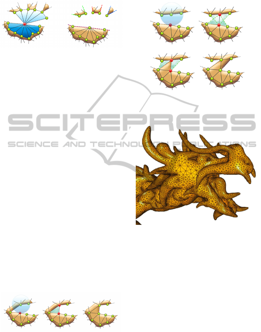
Figure 8: Cut out of a needle eye with a row of faces. Here,
each face is not necessarily connected to another face. In
contrast, if a needle eye has several groups of connected
faces then there are some omissions of faces around it.
normal can be seen as a direction pointing to the op-
posite side of the boundary. We define a sphere with
the center at c+n
c
r with radius r as the average length
of the edges at c
b
.
The coalescing condition at two boundaries hold,
i.e., merging of the boundaries containing c
b
and q on
the opposite side happens, if
• q is contained in the defined sphere, and
• scalar product of the boundary normals at c
b
and
q is negative.
Coalescing Process. After detecting the neural ver-
tex q to be connected with c
b
, the according faces
must be created starting with one edge from c
b
to q.
There are two cases which have to be considered.
Corner. A corner of the same boundary arises when
c
b
an q have one neighboring vertex in common (see
Fig. 9). A triangle of the three participating vertices
is created.
Long Side. Here, two boundaries appear to be
separated. After determining the new edge, there are
four possibilities for insertion of a new face contain-
ing the edge (see second picture in Fig. 10). The tri-
angle with edge lengths which vary fewest is taken in
our approach (see third picture in Fig. 10) since it is
the triangle with the best features concerning triangle
quality. Finally, to avoid a needle eye, a further tri-
angle must be added — again, we take the face with
Figure 9: Coalescing process at a mesh corner. On the left,
the search process of a coalescing candidate. In the middle,
one edge is created, on the right, the only face capable of
being added is the corner face.
Figure 10: Coalescing of two separate boundaries. In the
second picture, the edge is determined, in the third, the tri-
angle with smallest variance of edge lengths is added, in the
fourth, another triangle must be added to avoid a needle eye.
Figure 11: Roughness adaption correlates surface curvature
with mesh density, details of the model are exposed.
the greatest edge similarity (see fourth picture in Fig.
10).
2.2.3 Roughness Adaption
Up to now, the SGC are able to approximate an arbi-
trary sample set by a 2D mesh. What remains is an
efficient local adaption of the mesh density in a way
that areas with a strong curvature are modeled by a
finer mesh resolution (see Fig. 11). This also relieves
the influence of the sample density on the mesh gran-
ularity making the SGC less vulnerable to sampling
artefacts like holes or regions which are not sampled
with a uniform distribution.
Each time a vertex is adapted by a new sample we
calculate the estimated normal n
k
at a neural vertex
v
k
by the average of the normals at the surrounding
ICFC 2010 - International Conference on Fuzzy Computation
232

faces. The curvature c
k
∈ R at a vertex is determined
by
c
k
= 1 −
1
N
k
∑
∀n∈N
k
n
k
· n (1)
with the set N
k
containing the normals of the neigh-
boring neural vertices of v
k
. Each time a neural vertex
is selected as winner, its curvature value is calculated
and a global curvature value c is adjusted. Finally, the
curvature dependent resource term r
k
at v
k
is adapted
through r
new
k
= r
old
k
+ ∆r
k
, and
∆r
k
=
1, if (c
k
< c + σ
r
k
)
c
k
/(c + σ
r
k
)
(1 − r
min
) + r
min
else,
(2)
with the deviation σ
r
k
of the resource term r
k
, and a
constant resource r
min
that guarantees that the mesh
does not completely vanish at plane regions with a
very small curvature.
2.2.4 Curvature Cells
Each time after a vertex v
c
has been moved we apply
a smoothing mechanism like mentioned at the begin-
ning of section 2.2.
Roughness adaption (see section 2.2.3) leads to
the fact that in regions of high curvature the density
of neural vertices will increase. These vertices then
will get fewer sample hits, since they have a smaller
Voronoi region, and thus, Laplacian smoothing is ap-
plied fewer times.
We found out, that this significantly reduces mesh
quality in areas of high curvature. To avoid this, neu-
ral vertices in regions with high curvature are marked
as such and smoothing these is strengthened by re-
peating it n
L
times where
n
L
= b(c
k
− c)/σ
c
k
c − 1 (3)
with c
k
and c like defined in section 2.2.3 and σ
c
k
the
deviation of the curvature at vertex v
k
. The value is
limited to a maximum of N
L
to intercept looping at
extraordinary curvature values.
2.2.5 Discontinuity Cells
A sampled model that exposes discontinuities like
edges is difficult to be approximated by the neural net-
work mesh. Discontinuities are smoothed out since
the network tries to create a surface over them. This
might be acceptable in many application areas since
the approximation error is fairly small, but this effect
is unfavorable in computer graphics since it is clearly
visible. And even worse: edges are quite common in
real world scenarios.
Therefore, we propose discontinuity neural ver-
tices which, first, are only capable of moving in the
Figure 12: A dent (left picture) on a sharp edge is solved
(right picture) by an edge swap operation. Finally, connec-
tions of discontinuity vertices model object edges.
direction of an object edge to represent them more
properly, and second, the smoothing process is not ap-
plied to them.
Recognizing those vertices is accomplished as fol-
lows. We determine the curvature values of those
neighbors which have a distance of two connections
from the vertex (the “second ring” of neighbors).
Then the average δ
ring
of the squared differences of
consecutive curvature values on the ring is calculated.
If a curvature value clearly deviates from the av-
erage curvature value, then we assume that it is a
discontinuity vertex if the average of the neighbors’
(second ring) curvature gradient differs to a certain
amount. Thus, we define a vertex v
k
being a disconti-
nuity vertex if
(c
k
> 2σ
c
k
) ∧ (∀c ∈ C
k
: δ
ring
> 4σ
2
c
k
) (4)
with C
k
the set of curvature values of the second ring
of neighbors.
For approximating the edge normal we take the
average of the normals of two of the neighboring ver-
tices of v
k
, either those with the highest curvature
value, or those which are already marked as discon-
tinuity vertex. Finally, the normal is mirrored if the
edge angle lies above 180
◦
, which is indicated by the
average of the surrounding vertex normals; in the first
case it points in the direction of v
k
.
Edge swap. If two connected discontinuity vertices
grow into an edge, they nicely represent this edge by
a triangle edge. But if the line is interrupted by a non-
discontinuity vertex, a dent arises since this vertex is
not placed on the edge. Thus, we propose an edge
swap process which minimizes this effect.
Each time a discontinuity vertex is moved towards
a sample, the need for an edge swap operation will be
determined by collecting the three consecutive faces
with the most differing face normals. In case of a
dent, the face in the middle is assumed to be the one
which is misplaced and an edge swap operation is ap-
plied (see Fig. 12). Then, if the difference of the nor-
mals is now lower than before, edge swap is accepted,
if not, the former structure is held.
Edge swap results in models where finally edges
are represented by mesh boundaries (see Fig. 13).
SMART GROWING CELLS
233

2.2.6 Boundary Cells
Similar to discontinuity vertices which are capable of
moving to object edges, boundary vertices are able to
move to the outer border of a surface (see Fig. 14).
They are recognized by being part of a triangle edge
which is connected to one face only.
Then, these vertices are moved only in the direc-
tion of the boundary normal like described in section
2.2.2 in order to avoid vertices just lying in the aver-
age of the surrounding samples but directly match the
surface boundaries at their locations.
2.3 Results
For the full algorithm of this approach see the pseu-
docode in Fig. 16. To keep it comprehensive, the
outermost loop of the algorithm is neglected, and ver-
tex split and edge collapse operations are triggered by
counters.
Parameters which have been proven to be reliable
for almost all sample sets we took for reconstruc-
tion are ε
bm
= 0.1, ε
nb
= 0.08, r
min
= 0.3, ε
acute
=
0.5, n
degacute
= 4, k
ins
= 100, k
del
= 5, n
degnb
= 1,
n
nastyacute
= 4, n
nastyval
= 3.
The following results have been produced on a
Dell
R
Precision M6400 Notebook with Intel
R
Core 2
Extreme Quad Core QX9300 (2.53GHz, 1066MHz,
12MB) processor with 8MB 1066 MHz DDR3 Dual
Channel RAM. The algorithm is not parallelized.
Some visual results are exposed in Fig. 15. All
pictures are drawn from an SGC mesh. Most models
stem from the Stanford 3D Scanning Repository.
Besides visual results, reconstruction with SGC
comes up with impressive numbers compared to clas-
sical approaches, listed in table 1.
It can be seen that mesh quality, i.e. the percent-
age of perfect triangles in the mesh lies at 96% at
average. This is an outstanding result, nevertheless
this is usually expected when using an approach from
the field of unsupervised learning, since this guaran-
tees an ideal representation of the underlying training
Figure 13: Discontinuity vertices focus on edges. Edge
swap operations let mesh edges map to object edges.
Figure 14: Mesh boundary due to the missing bottom of the
statue is represented exactly by boundary cells.
Table 1: Results with sample sets from the Stanford
3D Scanning Repository. “Quality” means percent-
age of triangles which hold the Delaunay criterion.
RMS/Size is the root of the squared distances between
original point samples and the triangle mesh, divided
by the diameter of the sample set.
Samples Vertices
Time
[m:s]
Quality
RMS/
Size
36K 30K 0:39 95.6% 4.7e-5
438K 100K 2:47 95.5% 3.3e-5
544K 260K 9:15 93.1% 1.7e-5
14,028K 320K 12:17 98.5% 1.3e-5
5,000K 500K 21:5 95.9% 2.7e-5
511K 10K 0:11 99.8% 6.6e-5
38K 5K 0:6 99.0% 15e-5
346K 5K 0:6 98.3% 0.7e-5
sample distribution.
Further, the distance (RMS/object size) between
samples and mesh surface is negligible low — far be-
low 1% of the object size at average. This is even
more pleasant, since usually, the problem at edges
generate big error terms. Also the computing times
needed are very short, few minutes in each case.
All those measurements seem to be far better than
those from classical approaches, as long as we could
extract them from the regarding papers. Our algo-
rithm works very robustly. There are nearly no out-
liers visible in the mesh.
ICFC 2010 - International Conference on Fuzzy Computation
234
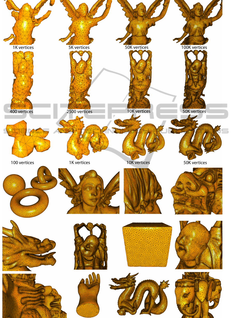
Figure 15: Upper lines: mesh training stages with number of vertices, lower lines, assorted pictures of reconstructed models.
SMART GROWING CELLS
235

Adjust samples regarding roughness.
Calculate average curvature and deviations.
Recognize and sign discontinuity cells.
Recognize and sign curvature cells.
for all Boundary cells do
if ∃ coalescing candidate then
Melt boundary.
for all Weeding candidates do
Weeding process.
end for
end if
end for
if Edge collapse operation triggered then
Collapse edge.
for all Weeding candidates do
Weeding process
end for
end if
if Vertex split operation triggered then
Split vertex.
end if
Figure 16: Outline of the complete SGC algorithm.
3 CONCLUSIONS
We presented a new neural network approach, the
smart growing cells, which is a modification of the
classical growing cells structures approach.
The modification type is new in a way that
it changes the pure, general unsupervised learning
scheme ad hoc to match training requirements of spe-
cific applications.
Thus, drawbacks of using unsupervised learning
approaches can be avoided while advantages be re-
tained, and nevertheless, SGC training keeps its roots
at general unsupervised learning.
We encourage this idea by one specific application
case — surface reconstruction from 3D point sam-
ples. Here, we add six topics to the classical unsuper-
vised learning scheme, and finally the approach out-
performs classical approaches concerning quality, ef-
ficiency, and robustness. Surface reconstruction with
SGC is able to handle arbitrary topologies and mil-
lions of samples. It recognizes and solves discontinu-
ities in the sample data and it is capable of adapting to
varying sample distributions. Finally, the network is
able to reorganize its topology to match arbitrary sur-
face structures. Altogether these advantages can not
be found in any of the classical approaches of surface
reconstruction.
The essential issue which transforms GCS to SGC
is the mechanism of weeding cells as a network clean-
ing mechanism for ill-formed structures. Further, face
normals are regarded and included in the neural net-
work training loop to adapt to mesh roughness and
to make the reconstruction process independent from
the sample distribution. Additionally, we propose co-
alescing cells which can connect to others, curvature
cells which recognize very small structures, and dis-
continuity cells which account for certain discontinu-
ous structures like sharp edges.
The proof of concept of our approach is enriched
by the achieved quality and performance measures.
For the tested geometries which each hold specific
challenges of reconstruction, we got approximation
errors for comparable mesh resolutions that lie far be-
low 1% at average. Mesh quality, measured by the
percentage of triangles which comply the Delaunay
criterion, lies at 96% at average. And the time needed
to compute meshes of several hundreds of thousands
of polygons were just few minutes.
Future Work. This work shows that application-
focused unsupervised learning is able to solve prac-
tical problems efficiently. Computation times are that
small that we think of a real-time reconstruction ap-
proach through multithreaded sample adjustment.
REFERENCES
Boissonnat, J.-D. (1984). Geometric structures for three-
dimensional shape representation. ACM Trans.
Graph., 3(4):266–286.
Edelsbrunner, H. and Mcke, E. P. (1994). Three-
dimensional alpha shapes.
Fritzke, B. (1993). Growing cell structures - a self-
organizing network for unsupervised and supervised
learning. Neural Networks, 7:1441–1460.
Fritzke, B. (1995). A growing neural gas network learns
topologies. In Tesauro, G., Touretzky, D. S., and Leen,
T. K., editors, Advances in Neural Information Pro-
cessing Systems 7, pages 625–632. MIT Press, Cam-
bridge MA.
Hoffmann, M. and Vrady, L. (1998). Free-form surfaces for
scattered data by neural networks. Journal for Geom-
etry and Graphics, 2:1–6.
Hoppe, H. (2008). Poisson surface reconstruction and
its applications. In SPM ’08: Proceedings of the
2008 ACM symposium on Solid and physical model-
ing, pages 10–10, New York, NY, USA. ACM.
Hoppe, H., DeRose, T., Duchamp, T., McDonald, J. A., and
Stuetzle, W. (1992). Surface reconstruction from un-
organized points. In Thomas, J. J., editor, SIGGRAPH,
pages 71–78. ACM.
ICFC 2010 - International Conference on Fuzzy Computation
236

Huang, Q.-X., Adams, B., and Wand, M. (2007). Bayesian
surface reconstruction via iterative scan alignment to
an optimized prototype. In SGP ’07: Proceedings of
the fifth Eurographics symposium on Geometry pro-
cessing, pages 213–223, Aire-la-Ville, Switzerland,
Switzerland. Eurographics Association.
Ivrissimtzis, I., Jeong, W.-K., Lee, S., Lee, Y., and Seidel,
H.-P. (2004a). Neural meshes: surface reconstruc-
tion with a learning algorithm. Research Report MPI-
I-2004-4-005, Max-Planck-Institut f
¨
ur Informatik,
Stuhlsatzenhausweg 85, 66123 Saarbr
¨
ucken, Ger-
many.
Ivrissimtzis, I., Jeong, W.-K., and Seidel, H.-P. (2003a).
Neural meshes: Statistical learning methods in surface
reconstruction. Technical Report MPI-I-2003-4-007,
Max-Planck-Institut fr Informatik, Saarbr
¨
ucken.
Ivrissimtzis, I., Lee, Y., Lee, S., Jeong, W.-K., and Seidel,
H.-P. (2004b). Neural mesh ensembles. In 3DPVT
’04: Proceedings of the 3D Data Processing, Visual-
ization, and Transmission, 2nd International Sympo-
sium, pages 308–315, Washington, DC, USA. IEEE
Computer Society.
Ivrissimtzis, I. P., Jeong, W.-K., and Seidel, H.-P. (2003b).
Using growing cell structures for surface reconstruc-
tion. In SMI ’03: Proceedings of the Shape Modeling
International 2003, page 78, Washington, DC, USA.
IEEE Computer Society.
Kohonen, T. (1982). Self-Organized Formation of Topolog-
ically Correct Feature Maps. Biological Cybernetics,
43:59–69.
Kolluri, R., Shewchuk, J. R., and O’Brien, J. F. (2004).
Spectral surface reconstruction from noisy point
clouds. In SGP ’04: Proceedings of the 2004 Euro-
graphics/ACM SIGGRAPH symposium on Geometry
processing, pages 11–21, New York, NY, USA. ACM.
MacQueen, J. B. (1967). Some methods for classification
and analysis of multivariate observations. In Pro-
ceedings of 5th Berkeley Symposium on Mathematical
Statistics and Probability, pages 281 – 297. University
of California Press.
Storvik, G. (1996). Bayesian surface reconstruction from
noisy images. In In Interface 96.
Taubin, G. (1995). A signal processing approach to fair
surface design. In SIGGRAPH, pages 351–358.
Vrady, L., Hoffmann, M., and Kovcs, E. (1999). Im-
proved free-form modelling of scattered data by dy-
namic neural networks. Journal for Geometry and
Graphics, 3:177–183.
Yoon, M., Lee, Y., Lee, S., Ivrissimtzis, I., and Seidel, H.-
P. (2007). Surface and normal ensembles for surface
reconstruction. Comput. Aided Des., 39(5):408–420.
Yu, Y. (1999). Surface reconstruction from unorganized
points using self-organizing neural networks. In
In IEEE Visualization 99, Conference Proceedings,
pages 61–64.
SMART GROWING CELLS
237
