AN ALGORITHM FOR DECISION RULES AGGREGATION
Adam Gudys and Marek Sikora
Institute of Computer Science, Silesian University of Technology, Akademicka 16, 44-100 Gliwice, Poland
Keywords: Decision rules, Decision rules aggregation, Knowledge discovery, Convex hull, Classification.
Abstract: Decision trees and decision rules are usually applied for the classification problems in which legibility and
possibility of interpretation of the obtained data model is important as well as good classification abilities.
Beside trees, rules are the most frequently used knowledge representation applied by knowledge discovery
algorithms. Rules generated by traditional algorithms use conjunction of simple conditions, each dividing
input space by a hyperplane parallel to one of the hyperplanes of the coordinate system. There are problems
for which such an approach results in a huge set of rules that poorly models real dependencies in data, is
susceptible for overtfitting and hard to understand by human. Generating decision rules containing more
complicated conditions may improve quality and interpretability of a rule set. In this paper an algorithm
taking a set of traditional rules and aggregating them in order to obtain a smaller set of more complex rules
has been presented. As procedure uses convex hulls, it has been called Convex Hull-Based Iterative
Aggregation Algorithm.
1 INTRODUCTION
Rules-based data models can be applied for the
classification (Furnkranz, 1999), description (Fayad
et al., 1996), or both the aims simultaneously. In the
case of description or both description and
classification, the possibility of interpretation of
created rules-based data descriptions, thus the ability
to understand and to use dependencies represented
by rules, is their significant feature. Due to the
specificity of the language of classification rules,
defining simple rules-based descriptions is
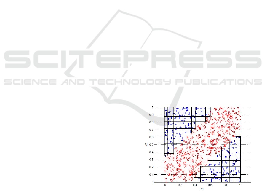
impossible for many problems (Fig. 1). It turned out
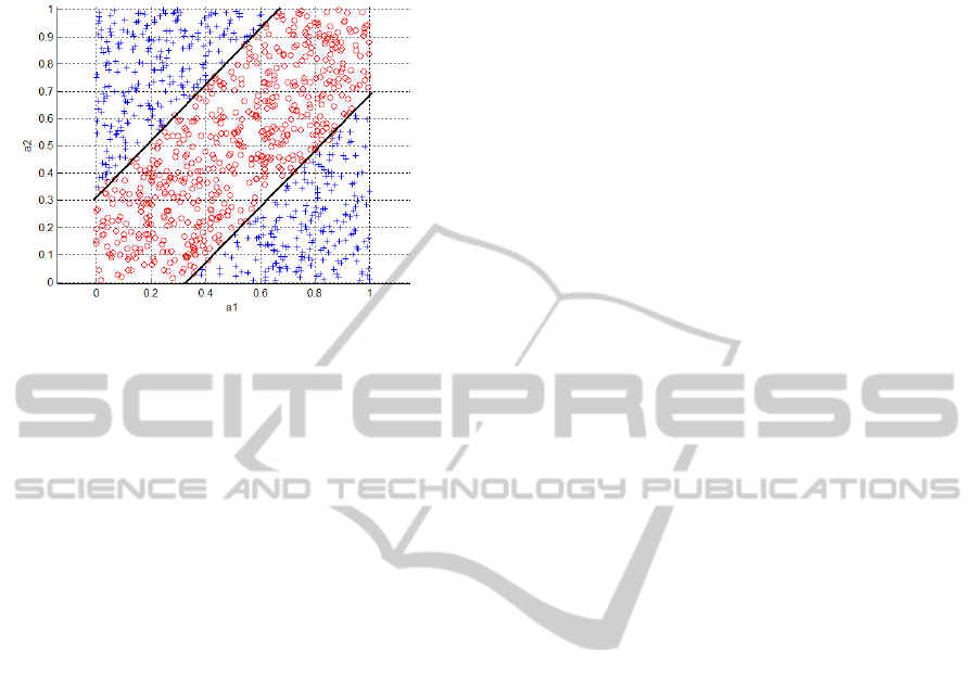
that if the language of rules representation is slightly
more complicated, simple and still intuitive
descriptions can be found for many of the problems
(Fig. 2). Therefore a lot of methods search for rules
which premises contain linear combinations of
conditional attributes. This enables to get so-called
oblique descriptors. The majority of the methods
make a decision trees induction (oblique decision
trees) (Murthy et al., 1994), (Bennett, Blue, 1997),
and then transform determined trees into rule sets.
The algorithm ARED (Seunghyun, Ras, 2008)
makes the rules induction with oblique descriptors.
However the efficiency of the algorithm was not
verified on a bigger number of datasets.
Figure 1: Example classification problem. Rules covering
decision regions have been induced using JRip which is an
implementation of the RIPPER algorithm (Cohen, 1995)
contained in Weka software (Hall et al., 2009). One can
see that the simple decision rule language is insufficient to
model the data properly.
Recently, an increasing number of hybrid rules
induction methods has been observed. Joining rules
induction algorithms with support vector machines
(SVM) is the most popular approach (Barakat,
Bradley, 2006), (Martens et al., 2009), (Nunez et al.,
2008). In the papers, SVM are usually used to
concentrate training examples on boundaries of
decision regions or to separate coherent regions in
the features space, and then describe them by rules
216
Gudys A. and Sikora M..
AN ALGORITHM FOR DECISION RULES AGGREGATION.
DOI: 10.5220/0003089702160225
In Proceedings of the International Conference on Knowledge Discovery and Information Retrieval (KDIR-2010), pages 216-225
ISBN: 978-989-8425-28-7
Copyright
c
2010 SCITEPRESS (Science and Technology Publications, Lda.)
with higher dimensional curves (e.g. ellipsoids) in
their premises.
Figure 2: Using a more complicated description language
allows to model classification problem nicely.
Each of the mentioned methods has advantages
as well as disadvantages. The fact that diagonal or
nonlinear descriptors occurring in rules apply all
conditional attributes without offering any pruning
strategies is the disadvantage in the majority of the
methods. The pruning is meant as simplifying multi-
dimensional expressions by eliminating conditional
attributes forming them. Possibility of interpretation
of unpruned rules is then strongly limited.
In the paper, a method of aggregating traditional
classification rules obtained by any standard rule
induction algorithm is presented. The procedure tries
to join rules sequentially, by twos, finding a set of
hyperplanes which bound a region covered by rules
being joined.
The presented method is a generalization of rules
joining algorithms which merge rules without
changing their representation language (Sikora,
2005), (Latkowski, Mikołajczyk, 2004) or operate
on a very specific representation (Pindur et al.,
2004).
In the next part of the paper, an algorithm for
rules aggregation and rules postprocessing, as well
as the results of experiments are presented. The last
chapter includes the summary of obtained results
and directions of further works.
2 BASIC NOTIONS
Some basic notions used later in the paper have been
introduced here.
Let's assume we have a set of objects O which
can be divided into c disjoint classes labelled by
elements of a set 1,2,…,. Information about
assignment of a given object o∈O to a decision class
is included in a value of a decision variable y:
:
1, 2,… ,
.
(1)
Let's additionally define a d-element set of attributes
,
,…,
. To each object
we
can assign a d-dimensional vector
,
containing values of
these attributes. One can see, that it has been
assumed that all the attributes from A are
continuous. This simplification is because the
current version of the algorithm ignores categorical
features in the aggregation process. However, a
generalization for categorical attributes is possible
and has been described later on.
A training set can be defined as follows:
, .
(2)
A classification task consists in finding a function ϕ
which approximates the function y on the basis of a
training set T (which is equivalent to generalising a
knowledge represented by a training dataset).
Rules-based classifiers can be distinguished by
classification strategies they exploit. Described
algorithm is based on a rules hierarchy. This is
because RIPPER algorithm (Cohen, 1995) which
served to generate input rules uses this scheme as
well. The idea is that rules are ordered. During the
classification process the first rule covering an
object being currently checked is picked. Hence,
reordering rules affects classification performance
(which is not the case in different aggregation
strategies like voting rules).
A decision rule can be defined as follows:
: ,
(3)
where is a premise consisting of a conjunction of
conditions (descriptors), and is a conclusion (a
class label). Majority of decision rules induction
algorithms generates simple descriptors like
or
. Such conditions divide an input space
into two parts by a hyperplane parallel to one of
hyperplanes of the coordinate system. Aggregation
algorithm covered in this paper generates oblique
descriptors, which are linear combinations of
attributes:
0.
(4)
Such descriptor divides a feature space by some
hyperplane, not necessarily parallel to coordinate
system hyperplanes. It is assumed, that inequalities
in all descriptors have the same direction (one can
always multiply expression by -1 to obtain this).
AN ALGORITHM FOR DECISION RULES AGGREGATION
217

Several measures that reflect a quality of
decision rules of the form (3) can be computed
(Furnkranz, Flach, 2005), (Guillet, Hamilton, 2007),
(Sikora, 2010). If the rule r is denoted as
ϕ
→
ψ
, then
n
ϕ
=n
ϕψ
+n
ϕ¬ψ
=|O
ϕ
| is the number of objects that
recognize the rule; n
¬ϕ
= n
¬ϕψ
+n
¬ϕ¬ψ
=|O
¬ϕ
| is the
number of objects that do not recognize the rule; n
ψ
=
n
ϕψ
+ n
¬ϕψ
=|O
ψ
| is the number of objects that belong
to the decision class described by the rule; n
¬ψ
=
n
ϕ¬ψ
+ n
¬ϕ¬ψ
=|O
¬ψ
| is the number of objects that do
not belong to the decision class described by the
rule; n
ϕψ
=|O
ϕ
∩O
ψ
| is the number of objects that
support the rule. Values n
ϕ¬ψ
, n
¬ϕψ
, n
¬ϕ¬ψ
are
calculated similarly as n
ϕψ
. It can be noticed that for
any rule
ϕ
→
ψ
the inequalities 1
≤
n
ϕψ
≤|O
ψ
|,
0≤n
ϕ¬ψ
≤|O
¬ψ
| hold. Hence, a quality measure is a
function of two variables n
ϕψ
and n
ϕ¬ψ
, and can be
defined as follows (Sikora, 2006):
ϕ
→
ψ
:1,..,|
ψ
|
×
0,..,|
¬ψ
|→.
(5)
Two basic quality measures are accuracy and
coverage:
acc(
ϕ
→
ψ
) = n
ϕ
ψ
/n
ϕ
,
(6)
cov(
ϕ
→
ψ
) = n
ϕ
ψ
/n
ψ
.
(7)
The accuracy measure and two other measures are
used for evaluation of joined rules in the aggregation
algorithm. The first measure called RSS is empirical
and enables to evaluate the accuracy and coverage of
a rule simultaneously, taking into consideration
examples distribution among the decision class
indicated by the rule and the other decision classes.
)(
ψϕ
→
Rss
q
=
1−
+
+
+
¬¬¬
¬¬
¬
ψϕψϕ
ψϕ
ϕψ
ϕψ
ϕψ
nn
n
nn
n
.
(8)
Making an analysis of the formula (8) it can be
noticed that the measure proposes the method of rule
evaluation analogous to the method of classifiers
sensitivity (first component of the sum) and
specificity (second component of the sum)
evaluation. The measure takes values from the
interval [-1,1] and values equal to zero are achieved
when a rule has the same accuracy as it implies from
the positive and negative examples distribution in a
training set.
The other measure used in a rule evaluation
process is Laplace estimate (9).
)(
ψϕ
→
Laplace
q
=
cnn
n
++
+
¬
ψϕϕψ
ϕψ
1
(9)
The basic idea of the Laplace estimate is to assume
that each rule covers a certain number of examples a
priori. The estimate computes the accuracy, but
starts to count covered positive or negative examples
at a number greater than 0. The positive coverage of
a rule is initialized with 1, while the negative
coverage of a rule is initialized with a number of
decision classes c.
3 CONVEX HULL-BASED
ITERATIVE AGGREAGTION
ALGORITHM
In the following paragraph an algorithm for
aggregation decision rules has been presented. It has
been called Convex Hull-Based Iterative
Aggregation Algorithm. Iterative, because it
sequentially tries to merge decision rules in order to
model the problem more properly than the input rule
set. Convex Hull-Based, because a procedure of
aggregating two particular decision rules uses
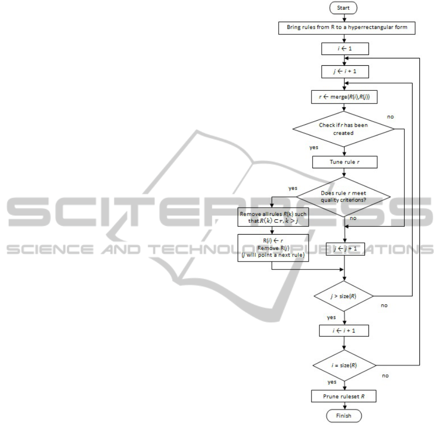
convex hulls. On the Fig. 3 one can see a full
flowchart of the algorithm. In the sections below all
steps of the procedure are covered in details.
Example dataset from the Fig. 1 has been used as an
illustration. One must keep in mind that it is
assumed, that input rule set R contains rules
corresponding to a single decision class.
3.1 Hyperrectangular Rules
The idea of the aggregation procedure is based on
the assumption that a decision rule can be
considered as some convex area in a feature space.
The algorithm tries to merge these areas into larger
ones. However, rules generated by traditional
induction algorithms rarely determine convex areas -
to obtain this, a rule should by bounded from both
sides in each dimension forming a hyperrectangle:
,
…
,
.
(10)
This is why the first step of the algorithm consists in
bringing an input rules into a hyperrectangular form.
This can be done by adding missing descriptors with
coordinates of the extreme points from a training set.
It will not affect classification results of unseen data
because these synthetically added descriptors will be
removed after aggregation procedure has finished. In
KDIR 2010 - International Conference on Knowledge Discovery and Information Retrieval
218
addition, hyperrectangular rules have a very nice
feature - one can easily find vertices of the
corresponding hyperrectangles. This is a crucial
issue because in the following steps algorithm uses
these vertices in the merging procedure. The
implication of the proposed approach is that a rule r
can be represented in a dual way:
• as a set of hyperplanes ,
• as a set of vertices .
Keeping integrity between the hyperplane
representation used directly for classification and the
vertex representation which takes part in the
aggregation procedure is a very important task the
algorithm must handle.
3.2 Aggregation Loop
As our aim is to reduce a number of rules in the
entire rule set meeting some classification accuracy
conditions, it must be decided which rules in which
order should be picked for the aggregation
procedure. The simplest approach is to use an
exhaustive paradigm to check all possible rule
permutations and pick the best one. However, the
brute-force method is computationally too expensive
to be used in practice. This is why some greedy
heuristics for searching aggregation candidates has
been proposed.
At the beginning we take the first rule as the
current one and try to merge it with following rules
(let's call those rules aggregation partners) creating a
candidates for new rules. Method of joining two
particular decision rules has been explained in the
following section. For each candidate we check if it
meets quality criterions.
Quality control consists of two elements. At first
algorithm checks how quality of the rule candidate is
related to the better rule from the pair being
aggregated. If it is below some threshold, the
candidate is rejected. Parameter indicating
maximum drop of the quality is called
ruleQualityDrop and is expressed in percentages.
However, checking only this condition may result in
an accumulation of the quality drops and big
classification error of the final rule set. This is why
an additional criterion has been introduced.
Algorithm checks how aggregation of two particular
rules affects classification accuracy obtained by the
entire rule set. If an accuracy decrease exceeds
rulesetAccuracyDrop parameter (which is given in
percentages as well), the candidate is rejected. One
must remember, that these two parameters are
evaluated on a training set. Adjusting them gives full
control on how the algorithm works. For example,
Figure 3: Flowchart of the Convex Hull-Based Iterative
Aggregation Algorithm.
one can force the algorithm to operate in the way
that classification accuracy obtained by a final rule
set does not decrease (on a training set).
If quality criterions are fulfilled, a rule candidate is
accepted. We replace the current rule with the new
one, and remove the partner from the rule set. The
algorithm also checks if the new rule covers some
other rules which follow the partner and removes
them if possible. There is no need to check rules
preceding the partner because they are the ones that
hasn't been aggregated with the current rule (so there
is no possibility that they are covered by the new
rule). After all partners have been checked, we
AN ALGORITHM FOR DECISION RULES AGGREGATION
219
change a current rule for the next one. Procedure
stops when the current rule is the last one from the
rule set.
3.3 Merging Two Decision Rules
This section covers in details how the algorithm
merges two particular decision rules. Let's assume
there are two rules
and
we would like to
aggregate. Below steps of the basic aggregation
procedure have been described. The modified
version with some improvements has been
introduced later.
1. Create a new rule r such that
.
2. Calculate a d-dimensional convex hull of
points belonging to the
using Qhull
algorithm (Barber et al., 1996). This
algorithm returns a set
describing all
the facets of a convex hull. Each facet is
represented by a set of d indices pointing
some vertices from
.
3. For each face from
calculate a
corresponding hyperplane equation.As we
know vertices belonging to each face, this
can be done easily by solving a system of
linear equations. Obtained hyperplanes are
stored in
set.
Important advantage of the method is that it can be
generalized for categorical attributes easily. Merging
descriptors
and
simply produces
. Another feature of the procedure is that
it is based only on rule vertices and does not use a
training set.
However, the approach described above has its
disadvantages. Most important one is that a number
of vertices representing a rule grows exponentially
with a number of dimensions. As hyperrectangular
rules use all attributes in their premises, handling
high dimensional feature spaces is computationally
very expensive. This is why, a hull should be
calculated only with respect to dimensions which are
really used in aggregated rules. Therefore, for each
input rule r, before bringing it to a hyperrectangular
form, we store attributes present in a premise in a set
. Additional improvement is to limit maximum
number of dimensions that can appear in a rule being
created. There is an algorithm parameter called
maxDim. If number of attributes in a rule candidate
exceeds this parameter, a rule is not created. This
allows user to control the complexity of obtained
(a)
(b)
Figure 4: Two hyperrectangular rules separately (a) and
after aggregation (b).
descriptors (for example, he can limit number of
dimensions to 3 in order to visualise hyperplanes) or
to speed-up the algorithm. The modified aggregation
procedure of rules
and
is as follows:
1. Create a new rule r such that
and
,
|
|
. If , reject r
immediately and skip the following steps.
2. Calculate a k-dimensional convex hull of
points from
with respect to the
attributes belonging to
. Following
actions are the same as in the previous
description.
The result of aggregation of two example rules has
been presented on the Fig. 4.
3.4 Rule Tuning
One can see on the flowchart that just after creation
of a new rule candidate there is a step called rule
tuning. It comes out that sometimes a rule candidate
may be further improved. This is very important
from the point of view of the algorithm because
quality influences if an aggregated rule is accepted.
KDIR 2010 - International Conference on Knowledge Discovery and Information Retrieval
220
Hence, each candidate is tuned to obtain as good
result as possible.
Rule tuning procedure has two phases. The first
stage of tuning consists in joining coplanar facets
and removing duplicated hyperplanes. As we
mentioned before, in k-dimensional space each facet
of a convex hull calculated by Qhull has k vertices.
This means that, for example, in 3-dimensional
space, we obtain triangular facets. Such approach
may result in coplanar facets. For example cube
contains 6 square facets but Qhull returns 12 triangle
ones. In fact, as our input rules have a
hyperrectangular form, this situation will happen
very often. More the dimensions, more coplanar
facets appear. This is why the algorithm must merge
coplanar facets and remove duplicated hyperplane
equations.
The second stage of tuning consists in adjusting
hyperplanes equations to get the maximum quality
of an aggregated rule. One can see on the Fig. 4 that
the oblique line is not optimally situated (if we
move it slightly upwards it will cover same number
of positive examples and less negative examples).
Hence, we introduce a technique of hyperplane
adjusting. For simplicity it is assumed that only
hyperplane translations are possible (no rotations are
performed). Below we described adjustment steps
for a rule r created as the result of aggregation of
rules
and
.
1. Find a hyperplane to adjust such
that
(there is no
need to improve a boundary hyperplane or a
hyperplane that could have already been
improved in one of previous iterations).
2. Find a face f corresponding to the
hyperplane h and all vertices from
adjacent to the face f. A vertex is adjacent
to the face f if it belongs to some face g
adjacent to f and it does not belong to f .
3. Calculate equations of hyperplanes parallel
to h going through vertices adjacent to f and
choose the one closest to h (let's call it
h
closest
). Original hyperplane h and the
closest one determine bounds of the
searching area. This is to assure that no face
vanishes in the adjustment procedure.
4. Use Fibonacci search technique (Ferguson,
1960) to find an optimal hyperplane h'
parallel to h lying in the area bounded by h
and h
closest
(as these hyperplanes are
parallel, Fibonacci is used to find an
optimal value of a free term). Assumed
quality measure is used as a criterion
function in searching.
5. Replace h with h' in , calculate new
positions of vertices forming face f using h'
equation and equations of adjacent faces.
This can be easily done by solving a system
of linear equations.
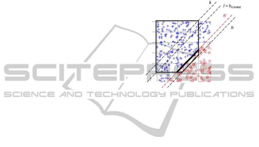
An example of the adjustment procedure has been
shown on the Fig. 5.
Figure 5: Tuning of a rule from the Fig. 4b. Hyperplane h
is the one being adjusted. Hyperplanes h and h
closest
indicate boundaries of the searching area. Hyperplane h' is
an optimal hyperplane found with Fibonacci method.
Adjusted face has been marked with a thick line.
3.5 Rule Set Pruning
Rule set pruning is done at the very end of the whole
procedure after the aggregation loop has finished.
This phase consists of actions that either decrease
rules quality (and should not be done in a tuning
phase preventing from a premature rejection of
candidates) or remove some data from a rule
description so further aggregations become
impossible.
There are two stages of pruning, both are
repeated for all rules in a rule set. First one consists
in eliminating hyperplanes that correspond to the
boundaries of the domain. As it has been said before,
the first step of the Iterative Aggregation Algorithm
is transforming input rules to the hyperrectangular
form. This means that some hyperplanes had to be
synthetically added. After the entire aggregation
procedure has finished, we can remove them.
The second stage of pruning consists in
removing other hyperplanes that have no significant
influence on classification results. Algorithm just
iterates through all the hyperplanes and checks how
deleting affects classifier performance. If a
classification accuracy decrease evaluated on a
training set does not exceed pruningAccuracyDrop
parameter (given in percentages), a hyperplane is
AN ALGORITHM FOR DECISION RULES AGGREGATION
221
removed. Below one can see a comparison between
some rule before and after pruning procedure.
Before pruning:
(-a1+0.602 >= 0) and
(-a1+0.432*a2+0.196 >= 0) and
(-a1+0.63*a2+0.022 >= 0) and
(-0.975*a1+a2-0.277 >= 0) and
(-0.491*a1+a2-0.329 >= 0) and
(-0.991*a2+1 >= 0) and
(+a2-0.348 >= 0) and
(+a1+0.01 >= 0) => class = positive
After pruning:
(-0.975*a1+a2-0.277 >= 0) =>
class = positive
As one can see, the reduction of descriptors number
is significant.
Actions described here cannot be done in the rule
tuning phase. This is because the hyperplane
adjustment procedure uses equations of adjacent
hyperplanes to calculate new positions of face
vertices. If one removed some hyperplanes from
, it would become impossible.
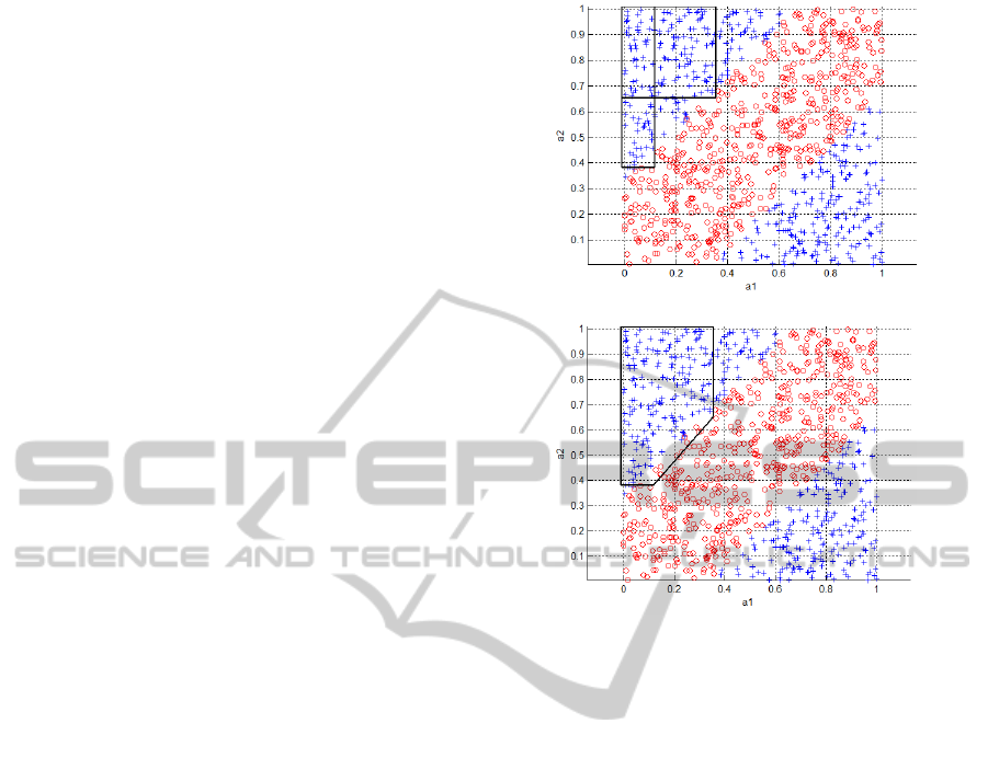
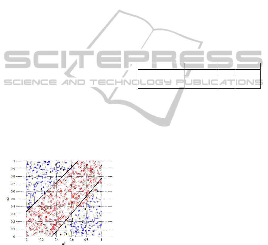
Final results of the algorithm for the example
input rule set has been shown on the Fig 6.
4 EXPERIMENTS
In order to evaluate results of the algorithm some
experiments have been performed. Benchmark
datasets have been chosen mainly from the UCI
Machine Learning Repository. The only exceptions
Figure 6: Final results of the Convex Hull-Based Iterative
Aggregation Algorithm performed on the rule set
presented on the Fig 1.
are synth2D (Fig. 1.) and synth3D datasets, which
have been synthetically generated and sc503 which
is the real dataset containing a microseismic hazard
assessment in a coal mine. Input rules have been
generated using JRip (Hall et al., 2009). Majority of
the experiments have been run in 10-fold cross
validation (only segment dataset has been tested in
the train and test mode). Tests have been performed
with four sets of parameters (from a very
conservative to a very aggressive aggregation
strategies) for the accuracy, RSS and Laplace quality
measures. In each experiment it has been checked
which measure leads to the best accuracy of an
obtained rule set and the best reduction of a number
of rules. Results are presented in the Table 1. One
can see that accuracy is the best quality measure if
we aim in the highest classification accuracy. If one
would like to reduce a number of rules, he should
pick RSS instead.
Table 1: Percentages indicate how often given quality
measure leads to highest accuracy and highest rule
reduction rate.
accuracy RSS Laplace
Highest accuracy 41% 29% 30%
Highest reduction
rate
24% 50% 26%
From all tested parameter sets we have chosen two
which haves been called safe and aggressive
aggregation strategies (see Table 2 for more detailed
description).
Tables 2a and 2b present results of
classification for these parameter sets for accuracy
and RSS quality measures respectively. This is due
to fact that these measures gave the best results from
the point of view of a classifier performance and a
rule set reduction. Results for Laplace have been
omitted, because they are located between accuracy
and RSS. One can see that results for the safe
strategy are similar for both quality measures.
However, in the aggressive strategy RSS leads to
lower accuracy and higher reduction of rule sets.
Below one can see a comparison between input
and output rules for “R” decision class for the
balance-scale data set. Aggressive parameter set has
been used with hyperplane dimensionality limitation
equal to 3. RSS has been set as a rule quality
measure.
KDIR 2010 - International Conference on Knowledge Discovery and Information Retrieval
222
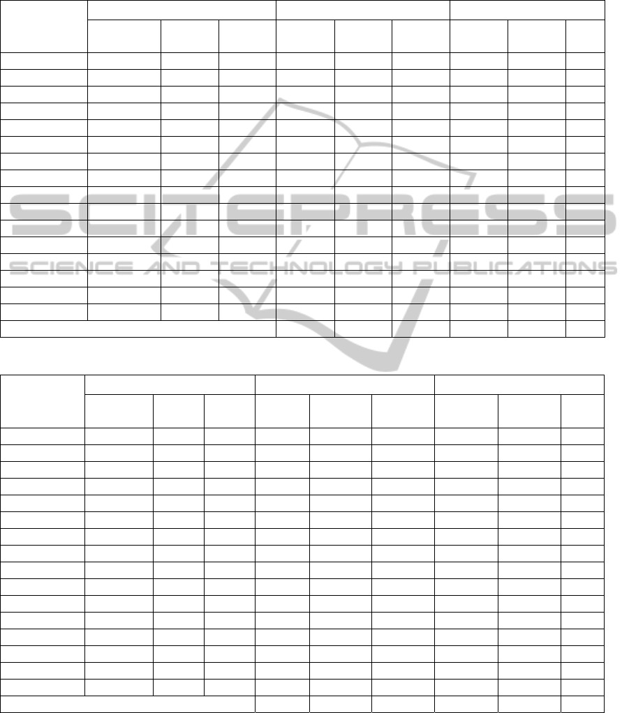
Table 2: Results of classification for the example datasets. Input rule set, and rule sets obtained by the safe and aggressive
aggregation strategies has been evaluated. Corresponding algorithm parameters are 20%-2%-1% and 20%-8%-2%
(ruleQualityDrop-rulsetAccuracyDrop-pruningAccuracyDrop). To speed up the calculations maximum number of
hyperplanes has been limited to 5. Accuracy (table a) and RSS (table b) have been used as quality measures.
(a)
Dataset
Input rule set Safe strategy Aggressive strategy
accuracy
[%]
rules
count
desc.
count
Δ(acc)
[%]
Δ(rc)
[%]
Δ(dc)
[%]
Δ(acc)
[%]
Δ(rc)
[%]
Δ(dc)
[%]
vehicle
67 16,7 42,1 2,3 -7,8 -32,5 0,6 -9 -37,5
wine
90,6 3,7 4,5 1,3 0 -2,22 1,3 0 -8,89
glass
65,4 7,2 14 1,3 -2,8 -7,86 1,5 -4,2 -12,1
iris
92,7 3,7 3,7 0,7 -5,4 -21,6 0,7 -5,4 -21,6
australian
84,1 4,7 8,7 1 -4,3 -14,9 1 -36 -67,8
pima
73,9 3,7 6,3 -0,4 -8,1 -19 -2 -19 -33,3
balance-scale
77,4 11,9 32,6 4,7 -81 -76,1 4,6 -81 -78,2
ionosphere
89,8 4,8 5,2 1 -10 -15,4 -1 -17 -25
heart-statlog
74,4 4 6,1 3 -40 -37,7 3 -43 -42,6
pendigits
86,7 30,8 75,1 -2 -12 -16,6 -4 -14 -18,6
ecoli
83 9,5 16,7 0,7 -6,3 -17,4 0,4 -7,4 -24,6
yeast
57,8 16,7 39,3 1,5 -14 -36,9 -0 -22 -47,8
segment
94,4 13 26 -0,5 -7,7 -15,4 -2 -7,7 -15,4
synth2D
95 10,9 19,8 2,3 -72 -86,4 1,7 -72 -87,9
synth3D
95,8 7,8 19,6 -1 -51 -61,2 -3 -60 -73,5
sc503
90,2 4,1 6,2 0,6 -22 -30,6 -1 -27 -40,3
Average 1,0 -21,5 -30,7 0,1 -26,5 -39,7
(b)
Dataset
Input rule set Safe strategy Aggressive strategy
accuracy
[%]
rules
count
desc.
count
Δ(acc)
[%]
Δ(rc)
[%]
Δ(dc)
[%]
Δ(acc)
[%]
Δ(rc)
[%]
Δ(dc)
[%]
vehicle
67 16,7 42,1 2,6 -16 -37,3 -3 -23 -48,5
wine
90,6 3,7 4,5 1,3 0 -2,22 1,3 0 -8,89
glass
65,4 7,2 14 0,6 -4,2 -9,29 -4 -11 -20
iris
92,7 3,7 3,7 0,7 -5,4 -21,6 0,7 -5,4 -21,6
australian
84,1 4,7 8,7 1 -6,4 -18,4 1 -36 -67,8
pima
73,9 3,7 6,3 -0,9 -11 -23,8 -2 -32 -50,8
balance-scale
77,4 11,9 32,6 6,5 -82 -76,7 5,6 -83 -79,1
ionosphere
89,8 4,8 5,2 0 -4,2 -7,69 -2 -19 -26,9
heart-statlog
74,4 4 6,1 3 -40 -37,7 3 -43 -42,6
pendigits
86,7 30,8 75,1 -2 -15 -16,5 -8 -23 -23,6
ecoli
83 9,5 16,7 0,7 -11 -20,4 -2 -17 -32,3
yeast
57,8 16,7 39,3 1,2 -28 -43,5 -1 -38 -60,1
segment
94,4 13 26 -0,5 -7,7 -15,4 -5 -23 -42,3
synth2D
95 10,9 19,8 2,2 -72 -86,9 2,1 -72 -87,9
synth3D
95,8 7,8 19,6 -1 -51 -57,7 -6 -71 -76,5
sc503
90,2 4,1 6,2 0 -27 -33,9 -1 -27 -38,7
Average 1,0 -23,8 -31,8 -1,3 -32,7 -45,5
AN ALGORITHM FOR DECISION RULES AGGREGATION
223

Input rule set:
(right-weight >= 3) and (right-distance
>= 3) and (left-weight <= 2) =>
class=R
(left-distance <= 2) and (right-weight
>= 3) and (right-distance >= 3) =>
class=R
(left-weight <= 3) and (left-distance
<= 2) and (right-weight >= 2) and
(right-distance >= 2) => class=R
(left-weight <= 1) and (left-distance
<= 3) and (right-distance >= 3) =>
class=R
(left-distance <= 1) and (right-weight
>= 3) and (left-weight <= 4) =>
class=R
(left-weight <= 1) and (right-distance
>= 2) and (right-weight >= 2) =>
class=R
(right-distance >= 4) and (right-weight
>= 4) and (left-weight <= 3) =>
class=R
(right-weight >= 5) and (right-distance
>= 4) and (left-weight <= 4) =>
class=R
(left-distance <= 3) and (right-weight
>= 3) and (right-distance >= 4) =>
class=R
(left-distance <= 3) and (right-weight
>= 4) and (right-distance >= 2)
and (left-weight <= 3) => class=R
(left-distance <= 1) and (right-weight
>= 2) and (right-distance >= 2) =>
class=R
(left-weight <= 3) and (left-distance
<= 1) and (right-distance >= 4) =>
class=R
Output rule set:
(-0.5*left-distance+1 >= 0) and
(+0.5*right-weight-1 >= 0) =>
class=R
(-0.5*left-weight+0.75*right-distance-
1 >= 0) and (+0.5*right-weight-1
>= 0) => class=R
(-0.333*left-distance+0.666*right-
weight-1 >= 0) and (+0.5*right-
distance-1 >= 0) => class=R
(-0.333*left-distance+1 >= 0) and
(+0.5*right-distance-1 >= 0) and
(+0.25*right-weight-1 >= 0) =>
class=R
(-left-distance+1 >= 0) => class=R
(-0.25*left-weight-0.25*left-
distance+1 >= 0) => class=R
One can see that rule reduction rate is significant.
The appearance of oblique descriptors allowed to
decrease the number of rules describing the training
data set and to reflect better dependences occurring
in the “R” decision class. Determined rules are
consistent with the balance scale dataset specificity.
In the case of the 2D synthetic dataset rules such
as in Fig. 6 were managed to obtain. It clearly shows
that the almost perfect description of the dataset has
been obtained. Obtaining the perfect one (as in the
Fig. 2) would be possible in the case of rotation of
one oblique descriptor by a certain angle. Such
tuning procedure will be the subject of further works
with the purpose of improving the algorithm.
5 CONCLUSIONS
The proposition of an algorithm for classification
rules aggregation that enables to introduce oblique
descriptors in rules premises is presented in the
paper. The aim of the algorithm is rules aggregation
in order to obtain less number of rules describing
decision classes. At the same time, the decrease of a
rules number should not influence negatively the
generalization abilities of the rules-based classifier.
Research results presented in tables 2a and 2b
show that the algorithm operates according to the
assumptions. Reduction of a number of rules and
descriptors occurring in their premises is the result
of the algorithm. The decrease of descriptors number
is obviously caused, among others, by the fact that
descriptors of aggregated rules can be linear
combinations of several attributes, so they are more
complicated than input ones. However, as the
example of the synthetic dataset presented in the
previous section shows, the change of descriptors
representation can be helpful in better understanding
dependencies in data.
The procedure tries to join rules sequentially, by
twos, finding a set of hyperplanes which limit a
region covered by rules being joined. Boundary
conditions added synthetically to premises of
aggregated rules are used in the hyperplanes
searching only.
The algorithm can be parameterized by using
various rule quality measures and various threshold
values connected with a quality of joined rules and
their classification abilities. As tables 2a and 2b
show, values of parameters are important for the
efficiency of the algorithm.
Further works on improving the algorithm
performance will concern developing more
advanced tuning strategy of joined rules. Beside the
method of a hyperplane translation, a strategy of its
rotation around a given point by a given angle will
be worked out. Probably, authors will take
KDIR 2010 - International Conference on Knowledge Discovery and Information Retrieval
224

advantage of experiences described by Murthy et al.
(1994).
The algorithm sources (written entirely in
MATLAB) can be provided after sending a request
to one of the authors.
ACKNOWLEDGEMENTS
This work was supported by the European
Community from the European Social Fund.
REFERENCES
Barakat, N., Bradley, A. B., 2006. Rule Extraction from
Support Victor Machines: Measuring the Explanation
Capability Using the Area under the ROC Curve. In
18th International Conference on Pattern Recognition.
Hong Kong, 2006.
Barber, C. B., Dobkin, D. P., Huh, H., 1996. The
Quickhull algorithm for convex hulls. ACM
Transactions on Mathematical Software, pp.469-83.
Bennett, K. P., Blue, J. A., 1997. A support vector
machine approach to decision trees. Department of
Mathematical Sciences Math Report No. 97-100.
Cohen, W. W., 1995. Fast effective rule induction. In
International Conference on Machine Learning.
Tahoe City, 1995. Morgan Kaufmann.
Fayad, U. M., Piatetsky-Shapiro, G., Smyth, P.,
Uthurusamy, R., 1996. From data mining to
knowledge discovery. In Advances in knowledge
discovery and data mining. Cambridge, 1996.
AAAI/MIT-Press.
Ferguson, D. E., 1960. Fibonaccian searching.
Communications of the ACM, December. p.648.
Furnkranz, J., 1999. Separate-and-conquer rule learning.
Artificial Intelligence Review, pp.3-54.
Furnkranz, J., Flach, P. A., 2005. ROC ‘n’ Rule Learning
– Towards a Better Understanding of Covering
Algorithms. Machine Learning, pp.39-77.
Guillet, F., Hamilton, H. J., 2007. Quality measures in
data mining. New York: Springer-Verlag.
Hall, M., Eibe, F., Holmes, G., Pfahringer, B., Reutemann,
P., Witte, I. H., 2009. The WEKA Data Mining
Software: An Update. SIGKDD Explorations.
Latkowski, R., Mikołajczyk, M., 2004. Data
Decomposition and Decision Rule Joining for
Classification of Data with Missing Values.
Transactions on Rough Sets I, pp.299-320.
Martens, D., Baesens, B., Gestel, T. V., 2009.
Decompositional Rule Extraction form Support Vector
Machines by Active Learning. IEEE Transaction on
Knowledge and Data Engineering, pp.178-91.
Murthy, S. K., Kasif, S., Salzberg, S., 1994. A system for
induction oblique decision trees. Journal of Artificial
Intelligence Research, pp.1-31.
Murthy, S. K., Kasif, S., Salzberg, S., 1994. A system for
induction oblique decision trees. Journal of Artificial
Intelligence Research 2, pp.1-31.
Nunez, H., Angulo, C., Catalia, A., 2008. Rule extraction
on support and prototype vectors. In J. Diederich, ed.
Rule extraction form SVM. Springer. pp.109-33.
Pindur, R., Susmaga, R., Stefanowski, J., 2004.
Hyperplane aggregation of dominance decision rules.
Fundamenta Informaticae, pp.117-37.
Seunghyun, I., Ras, Z. W., 2008. Action Rule Extraction
from a Decision Table: ARED. In ISMIS. Toronto,
2008. Lecture Notes in Computer Science.
Sikora, M., 2005. An algorithm for generalization of
decision rules by joining. Foundation on Computing
and Decision Sciences, Vol. 30, No. 3, pp.227-39.
Sikora, M., 2006. Rule Quality Measures in Creation and
Reduction of Data Rule Models. In Lecture Notes in
Artificial Intelligence Vol. 4259. Berlin Heidelberg:
Springer-Verlag. pp.716-25.
Sikora, M., 2010. Decision rules based data models using
TRS and NetTRS – method and algorithms.
Transactions on Rough Sets XI. Lecture Notes on
Computer Sciences Vol.5946, pp.130-60.
AN ALGORITHM FOR DECISION RULES AGGREGATION
225
