
TIME CONSTRAINTS EXTENSION ON FREQUENT SEQUENTIAL
PATTERNS
A. Ben Zakour, M. Sistiaga
2MoRO, Bidart, France
S. Maabout, M. Mosbah
Universit
´
e de Bordeaux, Bordeaux, France
Keywords:
Frequent pattern, Time constraint, Relax constraint, Sequential pattern mining.
Abstract:
Unlike frequent sets extraction for which only minimum support condition must be met, sequential patterns
satisfy time constraints. Commonly, to consider two events as successive, these constraints are either to respect
minimum and maximum time gap or to be included into a window size. In this paper, we introduce a new
definition of “interesting sequences”. This property suggests that temporal patterns, introducing concepts of
sliding window, can be customized by the user so that the events chronology in the extracted sequences has not
to strictly obey to the original event sequence.This definition is incorporated in the process of a conventional
algorithm (Fournier-Viger et al., 2008). The extracted patterns have an interval time stamp form and represent
an interesting palette of the original data.
1 INTRODUCTION
For Sequential Patterns Mining (SPM), the usage of
the temporal factor depends on the needs of this com-
ponent in the results. Existing extraction techniques
consider only the space component, the “succession”
of events in a sequence. In some cases, results can be
“exuberant” e.g., during the analysis of the shopping
basket, suppose that one customer buys product A and
product B a day later, and another one buys product A
and product B one month later. Based on these two
sequences, the pattern extracted is “a customer who
buys product A, buys the product B”. This conclu-
sion is not necessarily representative for the second
customer, and the extracted information is not repre-
sentative of the baseline data. Taking into account
the temporal aspect in the SPM was introduced in
(Srikant and Agrawal, 1996). Their constraints aim
to (1) bringing together “close” events into an indi-
vidual transaction and consider them as simultaneous
and (2) regulating the minimal and maximal time gaps
between two successive transactions. Considering the
importance of the temporal component in the inter-
pretation of patterns, (Hirate and Yamana, 2006) in-
troduce temporal constraints to extract temporal pat-
terns. They apply some improvements to Prefixspan
(Pei et al., 2004): (1) an interval function to upgrade
the timestamps of the bearing, (2) set the maximal and
minimal time gaps between two successive transac-
tions (3) min
whole interval and max whole interval
to regulate the minimum and maximum temporal
spread of a sequence. Both of these works intro-
duce time constraints to be satisfied by the extracted
sequences. One should notice that in both cases,
the extracted sequences respect the chronological or-
der that appears in the underlying data. However,
in some applications, close chronological ordering
is not necessary important for events. For example
the two temporal sequences h(0, A)(1, B)(2, C)i and
h(0, A)(1, C)(2, B)i may represent the same informa-
tion, that is A, B and C occur close to each other in
the interval [0,2]. The two algorithms presented pre-
viously do not consider this kind of information.
In this paper, we present a new definition of in-
teresting patterns. The idea is that we apply tempo-
ral relaxation on itemsets by using a backward sliding
window size constraint. Such a constraint can take
into account all neighbor events in a time window as
simultaneous.
The paper is organized as follows. First, we
present a brief state of the art. Then, we give a new
definition of interesting sequences. The third section
281
Ben Zakour A., Sistiaga M., Maabout S. and Mosbah M..
TIME CONSTRAINTS EXTENSION ON FREQUENT SEQUENTIAL PATTERNS.
DOI: 10.5220/0003098702810287
In Proceedings of the International Conference on Knowledge Discovery and Information Retrieval (KDIR-2010), pages 281-287
ISBN: 978-989-8425-28-7
Copyright
c
2010 SCITEPRESS (Science and Technology Publications, Lda.)

describes a modification of the algorithm presented
in (Fournier-Viger et al., 2008) to extract these se-
quences. A short evaluation of our approach is illus-
trated,a conclusion and perspectives in the last sec-
tion.
2 RELATED WORK
In this section, we present some general definitions
and two SPM works are detailed.
2.1 Terminology
A transaction is a timestamped itemset (or event
set). It is denoted by I
i
= {i
1
, i
2
, . . . , i
p
}. time(I
i
) de-
notes the timestamp of I
i
. A temporal sequence is a
timestamp ordered sequence of itemsets. It is denoted
by S = h(t
1
, I
1
), (t
2
, I
2
), . . . , (t
n
, I
n
)i where I
i
is a trans-
action and t
i
= time(I
i
). Hereafter, the timestamp t
i
is
related to the occurrence time of the first transaction
of the sequence. Thus, it represents the time lag be-
tween the transaction I
i
and I
1
. A sequence database
is a collection of sequences where each sequence has
a unique identifier id sequence. The support of a
sequence s in a sequence database SDB, denoted by
support
SDB
(s) is the percentage of sequences that
contain s in SDB. Given a minimal support minsupp,
s is frequent in SDB iff support
SDB
(s) ≥ minsup. Be-
sides minsupp and depending on the business needs,
the user may set time constraints that should be satis-
fied by the extracted patterns. The time constraints we
consider are: mingap and maxgap: represent respec-
tively the minimal and maximal time gap between two
successive transactions: time(I
i+1
) − time(I
i
) ≥ mingap
, time(I
i+1
) − time(I
i
) ≤ maxgap
Example 1. Let s = h(0, I
1
)(1, I
2
)(10, I
3
)i. If min-
gap=2 then transactions I
1
and I
2
are not considered
as successive because they are “too close”. If max-
gap is set to 5 then I
2
and I
3
are not considered as
successive because they are too distant.
min whole interval and max whole interval: rep-
resent respectively minimal and maximal whole
interval constraints. Let n be the number
of itemsets in a sequence. Then: time(I
n
) −
time(I
1
) ≥ min whole interval, time(I
n
) − time(I
1
) ≤
max whole interval
Example 2. Let min whole interval=1,
max whole interval=4 and s = h(0, I
1
)(1, I
2
)i. s
satisfies the min whole interval constraint and the
max whole interval constraint.
Window size: it allows to consider events (items)
in different transactions, such as simultaneous (within
a single transaction). These transactions should be
relatively close to each other regarding to the size of
the window.
Example 3. Let T = (0, AB) and s =
h(0, A)(2, B)(3, C)i. If ws=2 then s does contain
T while if window = 1, T is not contained in s.
2.2 GSP
In (Srikant and Agrawal, 1996), the authors improved
their A Priori algorithm (Agrawal and Srikant, 1994)
to bearing the absence of time constraint on timeless
patterns extracting. This algorithm relaxes transaction
definition by using a window notion and by integrat-
ing mingap and maxgap constraints.
Definitions. Let d = hd
1
d
2
...d
m
i and s = hs
1
s
2
...s
n
i
be two sequences. d contains the sequence s with con-
straint if and only if: Window size constraint : There
exist integers l
1
u
1
l
2
u
2
. . . l
n
u
n
such that:
s
i
⊆ ∪
u
i
k=l
i
d
k
, 1 6 i 6 n and time(d
u
i
) − time(d
l
i
) ≤
window size, 1 6 i 6 n mingap and maxgap con-
straints : There exist l
1
u
1
l
2
u
2
. . . l
n
u
n
such
that: s
i
⊆ ∪
u
i
k=l
i
d
k
, 1 ≤ i ≤ n, time(d
l
i
)−time(d
u
i−1
) ≥
mingap, for 2 ≤ i ≤ n and time(d
u
i
) − time(d
l
i−1
) ≤
maxgap, for 2 6 i 6 n. time(d
l
i
) is s
i
start time,
time(d
u
i
) refer to s
i
end time.
Algorithm Description. The main goal is to find
all frequent sequences satisfying all user constraints.
GSP is a level wise algorithm: first, it recovers L
1
the
set of frequent 1-sequences. It generates the candi-
dates sequences of size k + 1 by self-joining L
k−1
.
2.3 GSPM
(Hirate and Yamana, 2006) presents an approach for
extracting frequent temporal sequences from a tem-
poral sequences database. The algorithm applies time
constraints different from those applied in GSP. The
main goal is to extract temporal frequent patterns
from sequence database by integrating a new time
constraint that align interval timestamps into a same
value. The algorithm is an improvement of PrefixS-
pan (Pei et al., 2004) where data-sequences may be
either timestamped or just sorted.
Definition. Let f be a time function. It maps time
intervals to integers. Let f be defined as follows:
f (x) =
f
0
i f x ∈ [val
1
, val
2
[
f
1
is x ∈ [val
2
, val
3
[
...
f
n−1
i f x ∈ [val
n
, val
n+1
[
Let a = h(t
1
, X
1
), (t
2
, X
2
), . . . , (t
m
, X
m
)i and b =
h(t
0
1
, X
0
1
), (t
0
2
, X
0
2
), . . . , (t
0
n
, X
0
n
) be tow time sequences.
KDIR 2010 - International Conference on Knowledge Discovery and Information Retrieval
282

b is a subsequence of a w.r.t f , if and only if there
exist 1 ≤ i
1
i
2
... i
n
≤ m such that
• X
k
⊆ X
0
i
k
for all 1 ≤ i ≤ n and
• f (t
k
) = f (t
0
i
k
)
Let a sequence data base SDB, a sequence α =
h(t
1,1
, a
1
), (t
1,2
, a
2
), . . . , (t
1,m
, a
m
)i and X
β
an item-
set. If exist an Integer j (1 ≤ j ≤ m) as X
β
⊂ a
j
and I(t
1,β
) = I(t
1, j
), than the of α prefix regards
to X
β
, I(t
1,β
) is defined by: pre f ix(α, X
β
, I(t
1,β
)) =
h(t
1,1
, a
1
), (t
1,2
, a
2
)..., (t
1, j
, a
j
)i
The α suffix regards to X
β
, I(t
1,β
) repre-
sents sequence events those occurs after X
β
.
It’s defined by the: su f f ixe(α, X
β
, I(t
1,β
)) =
h(t
j, j
, a
0
j
), (t
j, j+1
, a
j+1
), . . . , (t
j,m
, a
m
)i.
Algorithm Description. The approach is a Prefixs-
pan extension (Pei et al., 2004). The first step is
to recover the frequent 1-sequences. Then, longer
patterns are extracted through a patterns growth pro-
cess. They are recovered by using a projection pro-
cess to discover, for each build patterns, the possible
continuations on the concerned set of the SDB. The
SDB projection on a α pattern is denoted by SDB|α
and defined by the equation: SDB|α = {is ∈ BD|is =
su f f ix(γ, 0, I)} avec γ ∈ SDB Iteration are stopped
when there is no possible continuation or no more fre-
quent items.
These two works extract frequent patterns by intro-
ducing time constraints. They relax the classical
transaction definition to better represent baseline data.
Relation is introduced through the application of the
grouping window size (Srikant and Agrawal, 1996)
and the temporal function in (Hirate and Yamana,
2006). Although those relaxation methods, it is im-
possible to associate unordered events.
In both methods, with a window size equals to
2 or with an equivalent time function, the se-
quence h(0, ABC)i does not contain the pattern
h(0, B)(1, AC)i. The algorithms look for item by item
and apply the projection, they keep as a continuation
only events that follow current item. In next section,
we present our approach which allows to take into ac-
count this kind of data.
3 INTERESTING SEQUENCES:
DEFINITIONS
In this paper, we propose to define a new type of inter-
esting sequences extracted from a temporal sequences
database. The difference with patterns extracted in
works presented, is the relaxation of transaction def-
inition without taking into account the order of items
within itmsets.
An “interesting sequence” is denoted by sp =
h(δt
1
, I
1
), (δt
1,2
, I
2
). . . , (δt
1,m
, I
m
)i. where I
i
is an
itemset . δt
1, j
is a transaction time stamp, it is the tem-
poral interval in witch I
j
events occur. This interval is
characterized by min time (respectively max temp),
its lower (resp. upper) bound. δt
1, j
is a relative times-
tamps w.r.t to I
1
occurrence where: min time and
max time are respectively the minimum and maxi-
mum time at which the events I
j
may occur after those
of I
1
.
Example 4. Let the sequence h(0, A)([2, 3], B)i
means that B occurs at earlier 2 times after A and
at the latest 3 times after A.
We consider the following time constraints:
• mingap and maxgap:
min(δt
i+1
) − max(δt
i
) ≥ mingap
max(δt
i+1
) − min(δt
i
) ≤ maxgap
• min whole interval and max whole interval:
min(δt
1
) − max(δt
n
) ≥ min whole interval
min(δt
1
) − max(δt
n
) ≤ max whole interval
• Window size:
max(δt
i
) − min(δt
i
) ≤ ws
Let s = h(t
1
, I
1
), . . . , (t
n
, I
n
)i and s
1
=
h(t
0
1
, s
1
), . . . , (t
0
m
, s
m
)i. s contains s
1
, denoted
s |= S
1
if and only if: For all 1 ≤ i ≤ m
s
1
⊂ (
F
l1
f
u=l1
d
I
u
), s
2
⊂ (
F
l2
f
u=l2
d
I
u
), . . . , s
m
⊂ (
F
lm
f
u=lm
d
I
u
)
max(time(
F
li
f
u=li
d
I
u
)) − min(time(
F
li
f
u=li
d
I
u
) ≤ ws
time(s
i
) ∈ [min(time(
F
li
f
u=li
d
I
u
)), max(time(
F
li
f
u=li
d
I
u
)]
min(time(
F
li+1
f
u=li+1
d
I
u
)) − max(time(
F
li
f
u=li
d
I
u
)) ≥ 0
Example 5. Let s
1
= h(0, A)(1, C)(2, B)(5, CDE)
(6, F)i, s
2
= h(0, AB)(5, FD)i and s
3
=
h(0, A)(12, CD)i. If window size ws is equal to
2, then s
1
contains s
2
. If mingap = 4 then s
1
does not
contain s
2
. Finally if maxgap = 10 then s
1
does not
contain s
3
: the gap between the maximal timestamps
of (CD) and the minimal time stamp of (AB) in s
3
is
greater than maxgap (12 ≥ 10).
This definition allows to extract patterns that can’t
be considered frequent by classical constraint. They
group, besides classical frequent patterns, those
grouping frequent unordered events occurring beside
a window interval.
4 COMPUTING INTERESTING
SEQUENCES
Problem Definition. Given a sequences
database, a support threshold minsupp, a window
TIME CONSTRAINTS EXTENSION ON FREQUENT SEQUENTIAL PATTERNS
283

size ws and time constraints: mingap, maxgap,
min whole interval and max whole interval, find all
interesting sequences.
Algorithm Description. The calculation of “inter-
esting” sequences is implemented through a modifi-
cation of the algorithm SPMF (Fournier-Viger et al.,
2008). This is an improvement of the algorithm Pre-
fixSpan (Pei et al., 2004). Initially, the algorithm ex-
tracts frequent items I from the sequences database.
This provides the set L
1
= {s
i
= (0, I)|support(I) ≥
minsupp}. Then, for providing continuations of each
1-sequence, SDB is projected onto each 1-sequence
(0, I). This projection is intended to take into account
the relaxation introduced by the window. The pro-
jection considers possible continuation of an event
that occurred at a time t. It backwards to event
occurring in the interval [ws − t, t] concatenated to
the “classical” continuation. This interval allows
to consider as possible “simultaneous” continuation
events appearing before the current event. Let α =
h(t
1,1
, a
1
), . . . , (t
1,m
, a
m
)i and a pair (δt, X
β
). If there
exists j such that 1 ≤ j ≤ m and X
β
⊂ a
j
and t
1,β
∈ δt
then the α prefix with regards to X
β
, t
1,β
is defined as:
wpre f ixe(α, X
β
, t
1,β
) =
h(t
1,1
, a
1
), (t
1,2
, a
2
), . . . , (t
1, j
, a
j
)i
The suffix of α wrt X
β
, I(t
1,β
) is defined as:
If j = 1 then wsu f f ix(α, X
β
, t
1,β
) = h(t
j, j
, a
j
\
X
β
), (t
j, j+1
, a
j+1
), . . . , (t
j,m
, a
m
)i, else it is equal to
h(t
j,k
, a
0
k
), . . . , (t
j, j
, a
j
\ X
β
), (t
j, j+1
, a
j+1
). . . , (t
j,m
, a
m
)i1 ≤
k ≤ m as t
jk
≤ ws and t
j(k−1)
≥ ws.
If j = 1 the projection of SDB on α = h(0, I)i is
defined by:
SDB|α = {ss = su f f ix(γ, I, ws)}, γ ∈ SDB
otherwise
SDB|α = {ss = wsu f f ix(γ, I, ws)}, γ ∈ SDB
The database projection on an item is described in Al-
gorithm 1. On each projection, frequent pairs are cal-
culated by using Find Frequent Pairs function. A
pair (δt, I) is a combination of a temporal interval and
an item. The interval is the period in which the item
occurs in the projection. The depth of this interval is
at most equals to the window size. Once a frequent
pair (δt, i) is identified, it is concatenated to the last
generated pattern. If the resulting pattern satisfies the
time constraints, then it is a new frequent sequence.
This new pattern generates a new iteration: the pro-
jection (SDB|α)|(δt, i) is computed and becomes the
new research space of frequent pairs.
Example 6. Let us consider example 5. The
projections of s
1
and s
2
w.r.t. h(0, A)i provide
resp. (SDB|
(0,A)
): s
1
: h(1, C)(2, B)(5, CDE)(6, F)i,
s
2
: h(0, B)(5, DF)i where the frequent pairs are:
([0, 2], B), ([5, 5], D), and ([5, 6], F).
size ws and time constraints: mingap, maxgap,
min whole interval and max whole interval, find all
interesting sequences.
Algorithm Description. The calculation of “inter-
esting” sequences is implemented through a modifi-
cation of the algorithm SPMF (Fournier-Viger et al.,
2008). This is an improvement of the algorithm Pre-
fixSpan (Pei et al., 2004). Initially, the algorithm ex-
tracts frequent items I from the sequences database.
This provides the set L
1
= {s
i
= (0, I)|support(I) ≥
minsupp}. Then, for providing continuations of each
1-sequence, SDB is projected onto each 1-sequence
(0, I). This projection is intended to take into account
the relaxation introduced by the window. The pro-
jection considers possible continuation of an event
that occurred at a time t. It backwards to event
occurring in the interval [ws − t, t] concatenated to
the “classical” continuation. This interval allows
to consider as possible “simultaneous” continuation
events appearing before the current event. Let α =
h(t
1,1
, a
1
), . . . , (t
1,m
, a
m
)i and a pair (δt, X
β
). If there
exists j such that 1 ≤ j ≤ m and X
β
⊂ a
j
and t
1,β
∈ δt
then the α prefix with regards to X
β
, t
1,β
is defined as:
wpre f ixe(α, X
β
, t
1,β
) =
h(t
1,1
, a
1
), (t
1,2
, a
2
), . . . , (t
1, j
, a
j
)i
The suffix of α wrt X
β
, I(t
1,β
) is defined as:
If j = 1 then wsu f f ix(α, X
β
, t
1,β
) = h(t
j, j
, a
j
\
X
β
), (t
j, j+1
, a
j+1
), . . . , (t
j,m
, a
m
)i, else it is equal to
h(t
j,k
, a
0
k
), . . . , (t
j, j
, a
j
\ X
β
), (t
j, j+1
, a
j+1
). . . , (t
j,m
, a
m
)i1 ≤
k ≤ m as t
jk
≤ ws and t
j(k−1)
≥ ws.
If j = 1 the projection of SDB on α = h(0, I)i is
defined by:
SDB|α = {ss = su f f ix(γ, I, ws)}, γ ∈ SDB
otherwise
SDB|α = {ss = wsu f f ix(γ, I, ws)}, γ ∈ SDB
The database projection on an item is described in Al-
gorithm 1. On each projection, frequent pairs are cal-
Algorithm 1: Projection.
Input: SDB, (δt, I)
foreach sequence s of SDB do
foreach itemset IS of s do
if I ∈ I
k
and t
k
∈ δt then
if IS r {I} =
/
0 then
add to projection
S = h((t
k
− ws), I
i
)...((t
k+1
−
t
k
), I
k+1
), ...((t
n
−t
k
), I
n
)i;
else
add to projection S =
h(t
k
−ws), I
i
)...(0, I
k
r{i}), ((t
k+1
−
tk), I
k+1
), ...((t
n
−t
k
), I
n
)i;
culated by using Find Frequent Pairs function. A
pair (δt, I) is a combination of a temporal interval and
an item. The interval is the period in which the item
occurs in the projection. The depth of this interval is
at most equals to the window size. Once a frequent
pair (δt, i) is identified, it is concatenated to the last
generated pattern. If the resulting pattern satisfies the
time constraints, then it is a new frequent sequence.
This new pattern generates a new iteration: the pro-
jection (SDB|α)|(δt, i) is computed and becomes the
new research space of frequent pairs.
Example 6. Let us consider example 5. The
projections of s
1
and s
2
w.r.t. h(0, A)i provide
resp. (SDB|
(0,A)
): s
1
: h(1, C)(2, B)(5, CDE)(6, F)i,
s
2
: h(0, B)(5, DF)i where the frequent pairs are:
([0, 2], B), ([5, 5], D), and ([5, 6], F).
For ([0, 2], B) iteration, the projection SDB|
([0,2],AB)
is: s
1
: h(−1, C)(3, CDE)(4, F)i, s
2
: h(5, DF)i where
frequent pairs are: ([3, 5], D), ([4, 5], F).
• For ([3, 5], D) iteration, the concatenation of
([0, 2], AB) and ([3, 5], D) is defined by:
– Items A and B are considered simultaneously
and take place in [0, 2].
– Item D is directly successive to AB and takes
place earlier than three time units after AB, so
D holds earlier than the time 5 = (2+3). More-
over, D occurs within 5 time units after AB, so
D will be held no later than the time 5 = (0+5).
Thus, the projection on ([3, 5], D) provides
SDB|
([0,2],AB)([5,5],D)
= s
1
: h(0, CE)(1, F)i, s
2
:
h(0, F)i.
The frequent pair ([0, 1], F). It provides the frequent
sequence: h([0, 2], AB)([5, 5], D)([5, 6], F)i and the
following projection: S
1
: h(−1, CE)i. There is no fre-
quent pair, so no new iteration is executed. The same
process is executed for the pairs ([4, 5], F)), ([5, 5], D)
and ([5, 6], F).
Conclusion. The approach we have presented pro-
vides frequent temporal patterns. Their timestamps
are in the form of intervals whose widths are ad-
justable by the user. These intervals allow a time oc-
currence approximation of events. As GSP (Srikant
and Agrawal, 1996), our approach uses also as input:
a set of sequences, support threshold and time con-
straints. The two main differences between both ap-
proaches are: (1) the extraction process used. The ef-
fectiveness of PrefixSpan over GSP was demonstrated
in various works (Fournier-Viger et al., 2008) (Hi-
rate and Yamana, 2006) (Pei et al., 2004). (2) the
quality of data. GSP patterns are timeless. In some
areas, lack of timestamps represents a major handi-
cap to data understanding and interpretation. In addi-
tion, the number of patterns returned by our approach
KDIR 2010 - International Conference on Knowledge Discovery and Information Retrieval
284

is more important. Indeed, the application of back-
ward window allows to expand continuation patterns
with those containing unordered events on a window
size interval. Then, where GSP considers no fre-
quent patterns, our approach searches through back-
ward window redundant information and extracts a
frequent pattern. The approach presented in (Hirate
and Yamana, 2006) has as input a sequences database,
a value of minsupp, time constraints and a time func-
tion to align timestamps. This approach and ours use
the same process of extracting patterns based on Pre-
fixSpan algorithm. The main difference concerns the
amount of data. While the use of the sliding window
can group events by degrees relative to the size of the
window, the function level has only the events whose
timestamps are in the same level. So, we end up with
more frequent patterns due to the sliding form of the
window, which groups gradually close events. Con-
crete results are presented in the next section.
Algorithm 2: Principal.
Input: SDB, minsupp, mingap, max gap,
min whole interval, max whole interval, ws,
Patterns
Patterns = null;
Find frequent items in SDB ;
foreach frequent item I do
prefix = (0, I);
SDB |
(0,I)
= Projection(SDB, (0,I), 0) ;
foreach pair (δt
f
, I
f
) in Find Frequent Pairs
(SDB|
(0,I)
, C1, C2) do
newprefix = concat(prefix, (δt
f
, I
f
));
if newprefix satisfies min whole interval and
max whole interval then
SDB|
(0,I)|(δt
f
,I
f
)
= Projection(SDB|
(0,I)
,
(t
f
, I
f
), ws) ;
Projection*(SDB|
(0,I)|(δt
f
,I
f
)
, minsupp,;
mingap, maxgap, min whole interval,;
max whole interval,
newF pre f ix, FSeq) ;
if newprefix 6∈ Patterns then
Add newprefix to Patterns ;
5 EXPERIMENTS
In this section, we present a qualitative experimenta-
tion of our approach. In a first part, the data used for
our experimentation are described. Then, we detail a
performance evaluation of the process used by the ap-
proaches, to motivate the method that we use to im-
plement our work. In a third part, we compare our im-
plementation to a GSPM implementation of patterns
growth process.
Algorithm 3: Projection*
Input: SDB, minsupp, mingap, maxgap,
min whole interval,
max whole interval, pre f ix, Patterns)
foreach Pair (f(t), t) in Find Frequent Pairs
(SDB, mingap, maxgap) do
newprefix = concat(prefix, (f(t),I));
if newprefix satisfies min whole interval and
max whole interval then
if support( f (t), I) ≥ minsupp then
Projection*(SDB|
( f (t)
p
,I
p
)
, mingap,
maxgap,;
min whole interval,
max whole interval,;
newprefix, patterns );
Add newprefix to Patterns;
Data Description. We applied our algorithms to real
aeronautical data related to a life history of six same
aircraft. These data represent missions, reports car-
ried out on different part of the vehicles and equip-
ments maintenance tasks execution. It is organized
on temporal sequences. A sequence is built by ac-
cumulating successive occurred events on an aircraft
between occurrence of a specific maintenance task.
Preprocessed sequences, from all vehicles and ended
with the application of a same maintenance task, rep-
resent lists of temporal events preceding the execu-
tion of the task. Extracting patterns from this database
consists in identifying commonly usages that lead to
the application of this maintenance task. It allows to
distinguish maintenance operations that use common
root causes. Table 1 represents a sequences history
sample for the task op m1. We used a GSP imple-
Table 1: Sample of preprocessed sequences.
ID Sequences
S 1 h(t=0, taxi, sale),(t=223, PARAPUB-
LIC, sandy ), (t=300, EMS, normal),
(t=330, report 1),(t=490, PARAPUB-
LIC, normal),(t=520, op m1)i
S 2: h(t=0, PARAPUBLIC, sandy), (t=190,
taxi,normal), (t=324, OEM, salt),
(t=500, op m1 ) i
S 3: h(t=0, EMS, normal), (t=190,taxi,salt),
(t=340, PARAPUBLIC, normal)(t=390,
report 1),(t=400 , op m1 )i
mentation available in WEKA
1
without any time con-
straints implementation. We also modified an imple-
mentation of (Fournier-Viger et al., 2008)
2
to obtain
the GSPM implementation. We modified the same
1
http://www.cs.waikato.ac.nz/ ml/weka/
2
http://www.philippe-fournier-viger.com/spmf
5 EXPERIMENTS
In this section, we present a qualitative experimenta-
tion of our approach. In a first part, the data used for
our experimentation are described. Then, we detail a
performance evaluation of the process used by the ap-
proaches, to motivate the method that we use to im-
plement our work. In a third part, we compare our im-
plementation to a GSPM implementation of patterns
growth process.
is more important. Indeed, the application of back-
ward window allows to expand continuation patterns
with those containing unordered events on a window
size interval. Then, where GSP considers no fre-
quent patterns, our approach searches through back-
ward window redundant information and extracts a
frequent pattern. The approach presented in (Hirate
and Yamana, 2006) has as input a sequences database,
a value of minsupp, time constraints and a time func-
tion to align timestamps. This approach and ours use
the same process of extracting patterns based on Pre-
fixSpan algorithm. The main difference concerns the
amount of data. While the use of the sliding window
can group events by degrees relative to the size of the
window, the function level has only the events whose
timestamps are in the same level. So, we end up with
more frequent patterns due to the sliding form of the
window, which groups gradually close events. Con-
crete results are presented in the next section.
Algorithm 2: Principal.
Input: SDB, minsupp, mingap, max gap,
min whole interval, max whole interval, ws,
Patterns
Patterns = null;
Find frequent items in SDB ;
foreach frequent item I do
prefix = (0, I);
SDB |
(0,I)
= Projection(SDB, (0,I), 0) ;
foreach pair (δt
f
, I
f
) in Find Frequent Pairs
(SDB|
(0,I)
, C1, C2) do
newprefix = concat(prefix, (δt
f
, I
f
));
if newprefix satisfies min whole interval and
max whole interval then
SDB|
(0,I)|(δt
f
,I
f
)
= Projection(SDB|
(0,I)
,
(t
f
, I
f
), ws) ;
Projection*(SDB|
(0,I)|(δt
f
,I
f
)
, minsupp,;
mingap, maxgap, min whole interval,;
max whole interval,
newF pre f ix, FSeq) ;
if newprefix 6∈ Patterns then
Add newprefix to Patterns ;
5 EXPERIMENTS
In this section, we present a qualitative experimenta-
tion of our approach. In a first part, the data used for
our experimentation are described. Then, we detail a
performance evaluation of the process used by the ap-
proaches, to motivate the method that we use to im-
plement our work. In a third part, we compare our im-
plementation to a GSPM implementation of patterns
growth process.
Algorithm 3: Projection*
Input: SDB, minsupp, mingap, maxgap,
min whole interval,
max whole interval, pre f ix, Patterns)
foreach Pair (f(t), t) in Find Frequent Pairs
(SDB, mingap, maxgap) do
newprefix = concat(prefix, (f(t),I));
if newprefix satisfies min whole interval and
max whole interval then
if support( f (t), I) ≥ minsupp then
Projection*(SDB|
( f (t)
p
,I
p
)
, mingap,
maxgap,;
min whole interval,
max whole interval,;
newprefix, patterns );
Add newprefix to Patterns;
Data Description. We applied our algorithms to real
aeronautical data related to a life history of six same
aircraft. These data represent missions, reports car-
ried out on different part of the vehicles and equip-
ments maintenance tasks execution. It is organized
on temporal sequences. A sequence is built by ac-
cumulating successive occurred events on an aircraft
between occurrence of a specific maintenance task.
Preprocessed sequences, from all vehicles and ended
with the application of a same maintenance task, rep-
resent lists of temporal events preceding the execu-
tion of the task. Extracting patterns from this database
consists in identifying commonly usages that lead to
the application of this maintenance task. It allows to
distinguish maintenance operations that use common
root causes. Table 1 represents a sequences history
sample for the task op m1. We used a GSP imple-
Table 1: Sample of preprocessed sequences.
ID Sequences
S 1 h(t=0, taxi, sale),(t=223, PARAPUB-
LIC, sandy ), (t=300, EMS, normal),
(t=330, report 1),(t=490, PARAPUB-
LIC, normal),(t=520, op m1)i
S 2: h(t=0, PARAPUBLIC, sandy), (t=190,
taxi,normal), (t=324, OEM, salt),
(t=500, op m1 ) i
S 3: h(t=0, EMS, normal), (t=190,taxi,salt),
(t=340, PARAPUBLIC, normal)(t=390,
report 1),(t=400 , op m1 )i
mentation available in WEKA
1
without any time con-
straints implementation. We also modified an imple-
mentation of (Fournier-Viger et al., 2008)
2
to obtain
the GSPM implementation. We modified the same
1
http://www.cs.waikato.ac.nz/ ml/weka/
2
http://www.philippe-fournier-viger.com/spmf
TIME CONSTRAINTS EXTENSION ON FREQUENT SEQUENTIAL PATTERNS
285
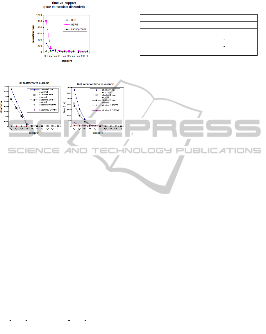
Figure 1: Process evaluation.
Figure 2: Performance evaluation.
code to implement our approach. First, we evaluate
the quality and results provided by our approach com-
pared to those provided by GSP. In a second step, we
evaluate the of performances cost of interesting se-
quences approach compared to GSPM, since the two
techniques are based on the same basic algorithm Pre-
fixSpan. We will then assess the quality of the results
of these two approaches.
Process Evaluation. We execute the three ap-
proaches by discarding time constraints to evaluate
the performance of allApriori method compared to
pattern-growth method. Figure 1 shows that execu-
tion time of pattern-growth (GSPM) is less than All
Priori( GSPM). These results reinforce our choice to
choose the Prefix Span approach.
Algorithm Evaluation. In this evaluation, we com-
pare execution time and the number of extracted se-
quences with varying minsupp. We compare SPMF
with backward window size, our proposed algorithm,
and generalized Sequential Patterns Mining with item
Interval. We have tested 3 situations:
situation 1 with f(t) = t/2, min gap= 3, max
gap = 5 and ws=2, situation 2 with f(t) = t,
min whole interval = 3, max whole interval = 7 and
ws = 0, situation 3 with f(t)=E(t/2), min gap= 1, max
gap = 5, min whole interval = 3, min whole interval
= 7 and ws = 2.
As shown in Figure 2(a), using our backward sliding
window allows to have a large number of patterns.
The number of extracted sequences increases expo-
nentially as minsupport decreases. Our approach is
Table 2: Result patterns.
GSPM results support
(fn(t)=0, taxi)(fn(t)=3, op m3 ) 0,5
Interesting sequences results
(t in [ 0.0, 0.0], taxi)(t in [ 2.0, 4.0], op m3) 1
(t in [ 0.0, 0.0], taxi)(t in [ 5.0, 7.0], op m3) 0,7
(t in [ 0.0, 0.0], taxi)(t in [ 4.0, 6.0], op m3) 0,8
interesting in high values of minsupport because it
provides patterns that are not extracted with GSPM.
For the lowest support values our approach execution
time is higher than that of GSPM (shown in Figure
2(b)). It is due to the greater number of possible con-
tinuations provided by the backward window size.
Patterns Quality Evaluation. Table 2 shows the
resulting patterns provided by GSPM in the first col-
umn and by our algorithm in the second one. We can
see that when GSPM provides a unique pattern our
approach shows 3 because of the sliding windows.
It allows the user to see all frequent possible com-
binations of patterns regarding to the user parame-
ters (windows size). So, our interesting sequences
approach has more exhaustive representation of the
data.
6 CONCLUSIONS
In this paper, we presented a new definition of in-
teresting sequences based on the principle of sliding
windows which takes into account any order within
transactions. This definition is important for sequence
data that do not require high timing precision. It al-
lows to gather as much information as possible to rep-
resent the actual data in a richer way without loss of
information. The definition presented here is inte-
grated into the process of the algorithm (Fournier-
Viger et al., 2008) and provides satisfying results
quality. Future work will focus on improving perfor-
mance. Another issue is the huge number of extracted
sequences. Extracting maximal interesting sequences
may be a solution to reduce the result size without
information loss. This approach is currently applied
on aeronautic vehicles life history to identify common
sequences preceding maintenance operations. These
same behaviors will be used for better maintenance
management and vehicle stops forecasting.
REFERENCES
Agrawal, R. and Srikant, R. (1994). Fast algorithms for
mining association rules in large databases. In VLDB
KDIR 2010 - International Conference on Knowledge Discovery and Information Retrieval
286

Proceedings.
Fournier-Viger, P., Nkambou, R., and Nguifo, E. M. (2008).
A knowledge discovery framework for learning task
models from user interactions in intelligent tutoring
systems. In Proceedings of the 7th MICAI Conf.).
Hirate, Y. and Yamana, H. (2006). Generalized sequential
pattern mining with item intervals. Journal of Com-
puters, 1(3).
Pei, J., Han, J., Mortazavi-Asl, B., Wang, J., Pinto, H.,
Chen, Q., Dayal, U., and Hsu, M. (2004). Mining
sequential patterns by pattern-growth: The prefixspan
approach. IEEE Trans. Knowl. Data Eng.
Srikant, R. and Agrawal, R. (1996). Mining sequential
patterns: Generalizations and performance improve-
ments. In Proc. of EDBT.
TIME CONSTRAINTS EXTENSION ON FREQUENT SEQUENTIAL PATTERNS
287
