THE

TYPHOON TRACK CLASSIFICATION USING TRI-PLOTS

AND MARKOV CHAIN

∗

John Chien-Han Tseng, Hsing-Kuo Pao

Research and Development Center, Central Weather Bureau, Taipei, Taiwan

Dept. of Computer Science & Information Engineering, National Taiwan University of Science & Technology, Taipei, Taiwan

Christos Faloutsos

Department of Computer Science, Carnegie Mellon University, Pittsburgh, PA, U.S.A.

Keywords:

Typhoon tracks, Trajectory data, ENSO, La Ni

na, Tri-plots, Markov chain, Dissimilarity measure, Isomap,

SSVM.

Abstract:

We aim at understanding typhoon tracks by classifying them into the ENSO and La Ni

na types. Two meth-

ods, namely, tri-plots and Markov chain combined with a novel dissimilarity measure for trajectory data are

proposed in this work. The calculation of the tri-plots can help us to separate ENSO from La Ni

na year ty-

phoon tracks with the training error about 0.023 to 0.268 and the test error about 0.271 to 0.334. The Markov

chain based dissimilarity measure, combined with the SSVM classiﬁer can help us to classify tracks with the

training error around 0.031 to 0.173 and the test error around 0.181 to 0.287. Moreover, for the purpose of

visualization, the tri-plots or Markov chain-based method maps the typhoon track data into low dimensional

space. In the space, the typhoon tracks of small dissimilarity should be regarded as one group. The map can

be very helpful for catching the hidden pattern of ENSO and La Ni

na atmospheric circulation for establishing

typhoon databases. In general, we believe that tri-plots and Markov chain-based method are useful tools for

the typhoon track classiﬁcation problem and should merit further investigation in related research community.

1 INTRODUCTION

It is an important and meaningful work of the typhoon

track classiﬁcation which can be used to diagnose

the atmospheric circulations and establish typhoon

databases. Some researches (Camargo et al., 2007a;

Camargo et al., 2007b; Lee et al., 2007) focused on

the different shapes or the clusters of the typhoon tra-

jectories. It means that they divide the typhoon tra-

jectories into several groups; for example, the east-

westward movement typhoons, or the recurved move-

ment having more north-southward component move-

ment typhoons, or maybe the typhoons close to the

continent, or the typhoons trapped in some areas,

etc. In general, they describe typhoon tracks mostly

based on their intuition without too much theoreti-

cal support. The method of Lee et al. (Lee et al.,

∗

Research

partially supported by Taiwan National Sci-

ence Council Grant # 98-2221-E-011-105.

2007) sliced the typhoon tracks into different seg-

ments by different moving directions, and used the

minimum description length (MDL) to cluster the ty-

phoon tracks. The method of Camago et al. (Ca-

margo et al., 2007a; Camargo et al., 2007b) followed

Gaffney and Smyth (Gaffney and Smyth., 1999) tra-

jectory clustering with mixtures regression models,

and arranged the typhoon tracks into seven clusters.

The common point of these researches regards every

single typhoon track as one sequence. In this work,

we consider typhoon tracks by collecting the typhoon

cases for a period of time to ﬁnd a global understand-

ing of the typhoon data. We examine the different

spatio-temporal structures of typhoon tracks for the

classiﬁcation.

In atmosphere, the most signiﬁcant annual circulation

variation events are ENSO (El Ni

no southern oscilla-

tion) and La Ni

na, the anti-ENSO. When the El Ni

or ENSO event happens, the anomaly of equatorial

364

Chien-Han Tseng J., Pao H. and Faloutsos C..

THE TYPHOON TRACK CLASSIFICATION USING TRI-PLOTS AND MARKOV CHAIN.

DOI: 10.5220/0003114303640369

In Proceedings of the International Conference on Knowledge Discovery and Information Retrieval (KDIR-2010), pages 364-369

ISBN: 978-989-8425-28-7

 2010 SCITEPRESS (Science and Technology Publications, Lda.)

sea surface temperature area will move to the central

Paciﬁc Ocean and that deﬁnitely causes the typhoon

generation area eastward and changes the shapes of

typhoon tracks. The purpose of this study is to clas-

sify the typhoon trajectories in a period of time into

either El Ni

no or La Ni

na event.

The method of tri-plots (Traina et al., 2001) is one

popular data mining tool to ﬁnd the patterns and re-

lationship between two large-scale, multidimensional

datasets. The tri-plots are composed of two self-

plots and one cross-plot. In the comparison of two

datasets through tri-plots, the two self-plots ﬁnd the

patterns of two individual datasets and the cross-plot

ﬁnds the relationship between the two datasets. Tak-

ing each El Ni

no and La Ni

na event data in turn, we

can depict the distribution of each data cloud by self-

plots and measure the distance of two data clouds by

cross-plots. We then use the distances from cross-

plots as the input for Isomap (Isometric feature map-

ping) (Tenebaum et al., 2000) to ﬁnd low-dimensional

embedding of the typhoon data. After that, in the low-

dimensional space, the smooth support vector ma-

chine (SSVM) with gaussian kernel (Lee and Man-

gasarian., 2001) is used to classify the typhoon data

into El Ni

no or La Ni

na event.

On the other hand, we propose a second method

for typhoon track classiﬁcation. We use Markov

chain (Bishop, 2006; Lin, 2009) to extract the hid-

den patterns of typhoon trajectories. We model a se-

quence, a period of time typhoon tracks, by a Markov

chain model. The consecutive time steps of the ty-

phoon coordinates can be described by conditional

probabilities in the Markov model. Risi (Risi, 2004)

also use Markov chain to analyze hurricane tracks,

but we focus on the classiﬁcation of typhoon tracks.

Moreover, we propose a novel dissimilarity measure

for a pair of sequences for typhoon track classiﬁca-

tion. Given two sequences, the dissimilarity measure

computes how well a sequence is described by the

model for another sequence and vice versa. Similarly,

the dissimilarity distance that we computed can be the

distances of the Isomap and the SSVM with gaussian

kernel is used for the classiﬁcation problem.

The remainder of this paper is organized as follows.

In Section 2, we introduce our typhoon dataset. Sec-

tion 3 and Section 4 in turn discuss the tri-plots and

the Markov chain-based dissimilarity measure for ty-

phoon track classiﬁcation, followed by their exper-

iment results. Then, in Section 5, we further dis-

cuss the proposed methods and summarize our con-

clusions.

2 DATA

The typhoon trajectory data that we discuss are

from Japan Meteorological Agency (JMA). The data

recorded the western Paciﬁc ocean which covers the

west of the longitude 180E to the east of the 100E ty-

phoon center movements (positions) and other obser-

vation variables, e.g., pressure, wind speed, etc. The

data features in this study include:

1. longitude,

2. latitude,

3. minimum pressure,

4. average high level (300 hPa) wind speed of the

typhoon center, and

5. topographical information.

We obtain the ﬁrst four features from the JMA

database; while the last topographical information is

calculated to show how close the typhoon center is

from the continent. The point is: when typhoon

touches the land, the intensity will decrease dramat-

ically or even disappear. Typhoon cannot hold longer

on the land, so it will not penetrate into the land so far.

In brief, if the typhoon center is at land, we deﬁne the

distance is equal to 0. In contrast, the typhoon center

is at sea, the distances between the center and the land

are calculated. Currently, the JMA data recorded the

typhoon trajectories from 1951 to 2009. The time res-

olution is about three to six hours. Furthermore, the

high level Meteorological data are from National Cen-

ter for Environment Prediction (NCEP) reanalysis-2

data. We use higher level (300 hPa) wind data in this

study, because the higher level wind steer the typhoon

movement (Chan and Gray., 1982; Emanuel, 2005).

The ENSO years and the La Ni

na years are based on

NOAAs (National Oceanic and Atmospheric Admin-

istration) deﬁnition by Ni

no 3.4 index. In order to

use the NCEP reanalysis-2 data, we only focus on the

time events after 1980. There are seven ENSO years

corresponding to seven ENSO events and the labels

are set to be 1 and there are ﬁve La Ni

na years as ﬁve

events and the labels are set to be −1 . We also have

ten neutral events which do not belong to either ENSO

or La Ni

na group. The number of labelled dataset

is relatively small. In some occasions, we chop the

events into sub-events so that we can obtain the result

with more statistical meaning.

THE TYPHOON TRACK CLASSIFICATION USING TRI-PLOTS AND MARKOV CHAIN

365

3 CLASSIFICATION BASED ON

TRI-PLOTS

Traina et al. (Traina et al., 2001) proposed the tri-plots

based on fractal dimension to calculate the difference

between two datasets. Given two datasets A and B, the

tri-plots can help us to judge whether the two datasets,

in this case, the ENSO and La Ni

na typhoon trajec-

tories, are from the same distribution. The tri-plots

include three kinds of plot tools:

1. self-plot ( for dataset A ),

2. self-plot ( for dataset B ), and

3. cross-plot ( for two datasets ).

For two datasets A and B, and the cross-plot function

is deﬁned by

Cross

A,B

(r) = log

∑

A,i

B,i

, (1)

where C

A,i

( C

B,i

) is the number of points from set

A( B ) in the i-th cell, and r is the distance for the pair

of points. Hence, the cross-plot function is propor-

tional to the count of A-B pairs within distance r, and

the cross-plot is the plot of the cross-plot function ver-

sus log(r). Moreover, the self-plot function is deﬁned

Sel f

(r) = log

∑

A,i

·(C

A,i

−1)

, (2)

and the self-plot is the plot of the self-plot function

versus log(r). If A is self similar, the self-plot of A

is close to a straight line and the slope is the intrin-

sic dimension of the set which is correlated with the

fractal dimension of the set (Belussi and Faloutsos.,

1995). In most situations, the cross-plot and self-plot

with log(r) are not linear, and we can use regression

method to determine the regression lines. We use

the line slopes to discuss the information between the

datasets A and B instead of the original data points.

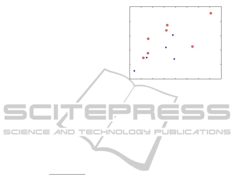
The Study of Self-plots. As mentioned, the fea-

tures that we used in this study are longitude, lati-

tude, minimum pressure, u (300 hPa), v (300 hPa),

and the topography information. The slope and in-

tercept based on self-plot function is regarded as the

point coordinates in a space. Then, we plot all the

annual ENSO and La Ni

na events in 2-D, as shown

in Figure 1. Basically, the ENSO points (red points)

and the La Ni

na points (blue points in the middle) are

roughly separated into two groups. It is interesting to

take a close look of the point set in the intercept verse

slope space. In Figure 1, we ﬁnd that the 8688 on the

top right and 9596 on the bottom left are two extreme

2.7 2.8 2.9 3 3.1 3.2 3.3 3.4 3.5

8.5

9.5

10.5

9596

0708

8485

9800

8889

0405

0203

9798

9495

9192

8688

8283

The distribution of (m,b) by 6−D (lon,lat,minp,u300,v300,Gauss_geo_dist) data points

slope

intercept

Figure 1: The slope and intercept of the tri-plots of typhoon

data. The longitude, latitude, minimum pressure, u (300

hPa), v (300 hPa) and topography effect are used in the ex-

periment. We can roughly observe that the ENSO points

(red points) and the La Ni

na points (blue points in the mid-

dle) are separated into two groups.

events. The 8688 event locates around the large slope

and intercept area; on the contrary, the 9596 event are

found around the small slope and intercept area. Af-

ter checking with the original typhoon trajectories, we

ﬁnd that the number of typhoon cases in 9596 is very

few and the number of cases is about 12 during this

period of time in contrast to other events. Meanwhile,

the number of typhoon cases in 8688 event is in nor-

mal situation, but it belongs to ENSO event and the

typhoons seem to travel longer distances than others.

When we use the distance to calculate the tri-plots,

the longer distances we get, the larger slope we have.

This explains why the 8688 event has large slope and

intercept and the 9596 event has small slope and in-

tercept.

We can check the Figure 1 following the vertical line

with the same slope; for example, along the lines

slope = 2.85 and slope = 3.1. There are two events,

9798 and 0203, located around the 2.85 slope; sim-

ilarly, there are two events, 8889 and 9800 located

around the 3.1 slope. When we check the typhoon

trajectories, it is easy to ﬁnd that the 8889 and 9800

events are very similar, and the 9798 and 0203 events

are very similar, too. As we know, the slope repre-

sents the fractal dimension, and the same fractal di-

mension of two data clouds implies that they are self-

similar. The different intercept but the same slope de-

picts that there are still differences in real geometrical

shapes; for example, a line and a circle (or a ring, i.e.,

without the inside part) have the same fractal dimen-

sion but different shapes. Based on this, the self-plot

distribution can afford a tool for atmospheric scien-

tists to do cluster studies.

KDIR 2010 - International Conference on Knowledge Discovery and Information Retrieval

366

The Study of Cross-plot. We would like to use

cross-plot to separate two types of data, the ENSO

and the La Ni

na typhoon trajectories. Based on

the same set of features, the output from the cross-

plot functions is regarded as the distances for the

Isomap. In Isomap (Tenebaum et al., 2000), we 1)

construct a neighborhood graph by linking each pair

of events/points that qualify as neighbors; 2) ﬁnd the

length of the shortest path between each pair of points

and take it as the approximation of their geodesic dis-

tance; and 3) take the pairwise (geodesic) distances

as the input and apply Multidimensional Scaling (or

MDS) to ﬁnd the global Euclidean coordinates of

the points. Because there are only 12 labeled events

(seven ENSO, ﬁve La Ni

na) in our study, it is not

so meaningful to operate the Isomap or the classiﬁ-

cation task based on such a small dataset. We split

the dataset from 12 events to 60 events by chopping

each of the original event into ﬁve smaller sub-events.

In here, we carefully chop the event so that one ty-

phoon case is still kept in the same event. We set

the intrinsic dimensionality (Tenebaum et al., 2000)

equal to ﬁve for Isomap, then classify the events by

SSVM in the embedded space produced by Isomap.

As shown in Table 1, the classiﬁcation results are:

training error around 0.023-0.268 and the test error

about 0.271-0.334, for different k’s for the nearest

neighbor choice.

Table 1: Error rates of the SSVM combined with cross-plots

and Isomap, for k equal to 5 to 10 which speciﬁes the num-

ber of closest neighbors used in the Isomap.

SSVM

5 6 7 8 9 10

training err. 0.27 0.03 0.12 0.03 0.02 0.03

test err. 0.33 0.27 0.36 0.29 0.32 0.33

4 CLASSIFICATION BASED ON

MARKOV CHAIN AND A

DISSIMILARITY MEASURE

We assume the typhoon trajectories can be repre-

sented as a sequence s = (x

,...,x

), where

is the coordinate value of typhoon center composed

of longitude and latitude at time t; the subscripts 1, 2,

. . . , T mean the different time stamps of the typhoon

positions. Then, we deﬁne the pace vector x

t+1

−x

and the Euclidean pace size λ

= kx

t+1

−x

k. So the

pace change is given by 4λ

= λ

t+1

−λ

. The angle

is deﬁned by the angle between vector x

t+1

−x

and the x-axis; and the angle change is given by

4θ

= θ

t+1

−θ

. Let m(σ

,σ

) denote the model

of trajectory sequence, and the transition parameters

are σ

, σ

which represent the standard deviation

of pace changes and angle changes. According to

Markov chain theory, the probability density func-

tion of 4λ

and 4θ

or the probability of having x

t+2

given x

t+1

can be described by

p(4λ

) ∼ N(4λ

mean

,σ

)

√

2πσ

exp

−

(4λ

−4λ

mean

)

2σ

(3)

p(4θ

) ∼ N(4θ

mean

,σ

)

√

2πσ

exp

−

(4θ

−4θ

mean

)

2σ

(4)

The log-likelihood `(s ; m) associated with trajectory

s and model m is written as

`(s; m) = log L(s ; m)

=log

p(x

)p(x

)

∏

t=1

P(x

t+2

t+1

)

=log p(x

) + log p(x

) +

∑

t=1

log(P(x

t+2

t+1

)).

(5)

We compute the (Shannon) code length of the trajec-

tory s as the negative log-likelihood as

c(s|m) = −`(s ; m) = −logL(s ; m). (6)

Finally, the dissimilarity value d is given by

d(s

) =

c(s

)

c(s

)

c(s

)

c(s

)

. (7)

In this equation, it estimates how effective if we want

to describe one trajectory by the model for other tra-

jectory. The dissimilarity matrix D can be given af-

ter calculating all the trajectory pairs d(s

). In this

study, in order to have representative typhoon trajec-

tories and save computing time, we combine several

typhoon tracks to be one trajectory. Because of com-

bining a period time typhoon trajectories as one se-

quence, the pace size between the ending point of one

trajectory and the beginning point of another trajec-

tory is larger than the regular pace sizes of consecu-

tive time stamps. We can choose the threshold with

4λ = 10 and ignore all the pace sizes of 4λ > 10.

We can compute two dissimilarity matrices D

4λ

and

4θ

based on two separated information about pace

size and angle and combine them into one target dis-

similarity as follows

target

= αD

4λ

+ (1 −α)D

4θ

, 0 ≤ α ≤1 (8)

In the formula, we can choose a larger α to respect

more of the importance of pace size information. In

THE TYPHOON TRACK CLASSIFICATION USING TRI-PLOTS AND MARKOV CHAIN

367

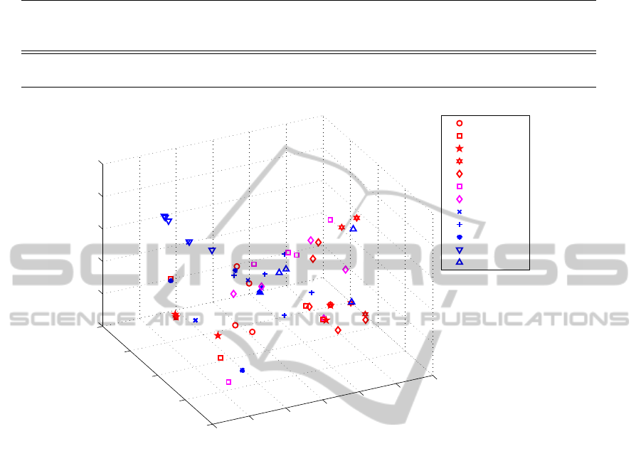
Table 2: The error rates of the SSVM based on Markov chain combined with the dissimilarity measure, with threshold

4λ ≤ 10 and k = 4 for the Isomap.

SSVM

0 0.1 0.2 0.3 0.4 0.5 0.6 0.7 0.8 0.9 1.0

training err. 0.17 0.05 0.14 0.06 0.16 0.17 0.15 0.04 0.03 0.04 0.05

test err. 0.28 0.25 0.25 0.22 0.29 0.29 0.28 0.20 0.18 0.20 0.25

−6

−4

−2

−4

−2

−1

enso0203

enso0405

enso8283

enso8688

enso9192

enso9495

enso9798

lanina0708

lanina8485

lanina8889

lanina9596

lanina9800

Figure 2: The 3-D structure from Isomap with k=4 based on the threshold 4λ ≤ 10 for the Markov Chain-based experiments,

with α = 0.8 in the dissimilarity matrix calculation.

Table 2, we can ﬁnd how different α’s can affect the

result. Again, we use SSVM following the Isomap for

the evaluation.

We want to compare the classiﬁcation result based on

tri-plots and the result combining the Markov chain

and the proposed dissimilarity measure. We separate

the original 12 events into 60 events using the same

data splitting method as the previous section. The

dissimilarity matrix D forms these 60 trajectories can

the input for the Isomap. Again, executing the SSVM

with the intrinsic dimensionality chosen to be ﬁve for

Isomap. The result is shown in Figure 2 and Table 2.

In Figure 2, we show the 3-D structure from Isomap.

The La Ni

na 9596 event located around left corner

with blue inverse triangle is the most different case

from the ENSO 8688 or ENSO 8283, and this result

is consistent with the tri-plots (Figure 1). Moreover,

the blue mark points on top left corner in Figure 2 are

from parts of La Ni

na cases like 8485, 8889, 9800

and 0708 which somehow show the trajectories close

to Asian continent. Based on 10-fold cross validation,

the training error is 0.031-0.173 and the test error is

around 0.181-0.287.

5 CONCLUSIONS AND FUTURE

WORKS

In this study, we proposed the quantitative and objec-

tive tools, tri-plots and Markov chain-based method,

to distinguish the differences between the different

yearly typhoon track events. Based on the evaluation,

we have about 70% accuracy on classifying the ty-

phoon tracks belonged to El Ni

no or La Ni

na events.

In tri-plots, we afford a global view to see different

annual events by the self-plot distribution, and the re-

sult is consistent with the report of World Meteoro-

logical Organization (World Meteorological Organi-

zation, 2009), that is, no two El Ni

no events are iden-

tical. Moreover, the self-plot distribution affords the

information for future clustering studies of El Ni

KDIR 2010 - International Conference on Knowledge Discovery and Information Retrieval

368

and La Ni

na events. Besides, the tri-plots experiments

tell us what kind of features we probably should have

them included for the classiﬁcation or for typhoon

databases. Until now, the world typhoon databases

just store the low level features of typhoons. We be-

lieve that adding the high level winds or the consid-

eration of topographical effect should be included in

typhoon databases. On the other hand, the Markov

chain-based model gives us better performance than

the tri-plots. However, the different probability dis-

tributions should be considered in the future, that is,

Markov chain-based model still has more potential to

do the following classiﬁcation researches. Finally, ei-

ther tri-plots or different Markov chain models, can

be extended to other traditional Meteorological data

analysis. Because the quantity of the Meteorologi-

cal is very large; for example, the space resolution

of NCEP reanalysis data is about 144×73 in hori-

zontal; the 17 layers in vertical for one speciﬁc fea-

ture and the time resolution is about 4 times in one

day. So, when we extend our methods to analyze the

annual events, we need to modify our current algo-

rithm. First, we need an alternative method to solve

the eigenproblem in Isomap (solving large and sparse

matrix), and we need more efﬁciency box-counting

data structure in tri-plots.

REFERENCES

Belussi, A. and Faloutsos., C. (1995). Estimating the se-

lectivity of spatial queries using the correlation fractal

dimension. pages 299–310. In the 21-th conference of

Very Large Data Bases.

Bishop, C. M. (2006). Pattern recognition and machine

learning. Springer press.

Camargo, S, J., Robertson, A. W., Gaffney, S. J., and Smyth,

P. (2007a). Cluster analysis of typhoon tracks. Part

I: general properties. Journal of Climate, 20:3635–

3653.

Camargo, S, J., Robertson, A. W., Gaffney, S. J., and Smyth,

P. (2007b). Cluster analysis of typhoon tracks. Part

II: large circulation and ENSO. Journal of Climate,

20:3654–3676.

Chan, J. C. L. and Gray., W. M. (1982). Tropical cy-

clone movement and surrounding ﬂow relationships.

Monthly Weather Review, 100:1354–1374.

Emanuel, K. (2005). Divine wind: the history and science

of hurricanes. Oxford university press.

Gaffney, S. and Smyth., P. (1999). Trajectory clustering

with mixtures of regression models. pages 63–72. In

the International Conference on Knowledge Discov-

ery and Data Mining.

Harr, P. A. and Elsberry, R. L. (1991). Tropical cy-

clone track characteristics as a function of large-

scale circulation anomalies. Monthly Weather Review,

119:1448–1468.

Hsieh, W. (2009). Machine learning methods in the envi-

ronmental sciences. Cambridge university press.

Jordan, M. I. An introduction to probabilistic graphic mod-

els. In preparation.

Lee, J.-G., Han, J., and Whang., K.-Y. (2007). Trajectory

clustering: A partition-and-group framework. pages

593–640. International Conference on Management of

Data.

Lee, Y.-J. and Mangasarian., O. L. (2001). SSVM:

A smooth support vector machine for classiﬁcation.

Comput. Optim. Appl., 20(1):5–22.

Lin, H. (2009). Trajectory based on behavior analysis for

veriﬁcation and recognition. Master’s thesis, National

Taiwan University of Science and Technology, master

thesis, Taipei.

Miller, J., Weichman, P. B., and Cross, M. C. (1992). Statis-

tical mechanics, eulers equation, and jupiters red spot.

Physics Review, A45:2328–2359.

Risi, C. (2004). Statistical synthesis of tropical cyclone

tracks in a risk evaluation perspective. Technical re-

port, Massachusetts Institute of Technology, intern-

ship report, Cambridge.

Strogatz, S. H. (2001). Nonlinear dynamics and chaos: with

applications to Physics, Biology, Chemistry, and engi-

neering. Westview press.

Tenebaum, J. B., d. Silva, V., and Langford., J. C. (2000). A

global geometric framework for nonlinear dimension-

ality reduction. Science, 290:2319–2323.

Traina, A., Traina, C., Papadimitriou, S., and Faloutsos, C.

(2001). Tri-plots: Scalable tools for multi dimensional

data. pages 184–193. In the International Conference

on Knowledge Discovery and Data Mining.

Vlachos, M., Gunopulos, D., and Kollios, G. (2002). Dis-

covering similar multidimensional trajectories. pages

673–684. In the International Conference on Data En-

gineering.

Wang, B., Rui, H., and Chan, J. C. L. (2002). How strong

ENSO events affect tropical activity over the western

north paciﬁc. Journal of Climate, 15:1643–1658.

Webster, P. J., Holland, G. J., Curry, J. A., and Chang., H.-

R. (2005). Changes in tropical cyclone number, dura-

tion, and intensity in a warming environment. Science,

309:1844–1846.

World Meteorological Organization (2009). El Ni

no/La

na update. Technical report, World Meteorological

Organization.

THE TYPHOON TRACK CLASSIFICATION USING TRI-PLOTS AND MARKOV CHAIN

369