
* Venkata Praveen Karri did this work when he was at
University of North Texas.
EFFECTIVE AND ACCELERATED INFORMATIVE FRAME
FILTERING IN COLONOSCOPY VIDEOS USING GRAPHICS
PROCESSING UNIT
Venkata Praveen Karri*, JungHwan Oh
Department of Computer Science and Engineering, University of North Texas, Denton, TX 76203, U.S.A.
Wallapak Tavanapong, Johnny Wong
Computer Science Department, Iowa State University, Ames, IA 50011, U.S.A.
Piet C. de Groen
College of Medicine, Mayo Clinic, Rochester, MN 55905, U.S.A.
Keywords: Colonoscopy, CUDA, GPU, CPU multi-threading, Informative frame filtering.
Abstract: Colonoscopy is an endoscopic technique that allows a physician to inspect the mucosa of the human colon.
It has contributed to a marked decline in the number of colorectal cancer related deaths. However, recent
data suggest that there is a significant (4-12%) miss-rate for the detection of even large polyps and cancers.
To address this, we have investigated automated post-procedure and real-time quality measurements by
analyzing colonoscopy videos. One of the fundamental steps is separating informative frames from non-
informative frames, a process called Informative Frame Filtering (IFF). Non-informative frames comprise
out-of-focus frames and frames lacking typical features of the colon. We introduce a new IFF algorithm in
this paper, which is much more accurate than our previous one. Also, we exploit the many-core GPU
(Graphics Processing Unit) to create an IFF software module for High Performance Computing (HPC).
Code optimizations embedded in the many-core GPU resulted in a 40-fold acceleration compared to CPU-
only implementation for our IFF software module.
1 INTRODUCTION
Colonoscopy is an endoscopic technique that allows
a physician to inspect the mucosa of the human
colon. It has contributed to a marked decline in the
number of colorectal cancer related deaths
[American Cancer Society, 2008]. However, recent
data suggest that there is a significant (4-12%) miss-
rate for the detection of even large polyps and
cancers [Johnson, D., et al. 2007, Pabby, A., et al.
2005]. To address this, we have been investigating
two approaches. One is to measure post-procedure
quality automatically by analyzing colonoscopy
videos captured during colonoscopy. The other is to
inform the endoscopist of possible sub-optimal
inspection immediately during colonoscopy in order
to improve the quality of the actual procedure being
performed. To provide this immediate feedback, we
need to achieve real-time analysis of colonoscopy
videos.
A fundamental step of the above two approaches
is to distinguish non-informative frames from
informative ones. An informative frame in a
colonoscopy video can be broadly defined as a
frame which is useful for convenient naked-eye
analysis of the colon (Figure 1). A non-informative
frame has the opposite definition (Figure 2). In
general, non-informative frames can be considered
out-of-focus frames. Our intention is not to increase
the sharpness of these frames (which is commonly
known as 'auto-focusing technique'), but to just filter
them out.
Informative and non-informative frames can be
loosely termed as clear and blurry frames
respectively. But, these loose definitions are not
sufficient for proper frame filtering in colonoscopy
video. In a colonoscopy context, the definition of
119
Karri V., Oh J., Tavanapong W., Wong J. and de Groen P..
EFFECTIVE AND ACCELERATED INFORMATIVE FRAME FILTERING IN COLONOSCOPY VIDEOS USING GRAPHICS PROCESSING UNIT.
DOI: 10.5220/0003123401190124
In Proceedings of the International Conference on Bio-inspired Systems and Signal Processing (BIOSIGNALS-2011), pages 119-124
ISBN: 978-989-8425-35-5
Copyright
c
2011 SCITEPRESS (Science and Technology Publications, Lda.)
informative and non-informative frames is slightly
different from the conventional definition of clear
and blurry images. We presume that a typical
informative frame in colonoscopy is primarily
characterized by curvaceously (circular or semi-
circular) connected vivid lines (not just any lines
like horizontal, vertical or broken lines), because
that is the typical content of an informative colon
frame (Figure 1(d)). Curvaceous connectivity means
more connectivity in diagonal and circular
directions. Our intention is to retain frames which
satisfy this definition and to filter out the rest. The
best way to completely realize this definition is
firstly to detect the presence of such vivid lines, and
secondly to measure the amount of curvaceous
connectivity they possess. Then, with the help of a
carefully chosen threshold, we identify frames which
exhibit more curvaceous connectivity and classify
them as informative, and vice-versa. In this paper,
we propose a highly accurate algorithm for this
informative frame filtering (IFF).
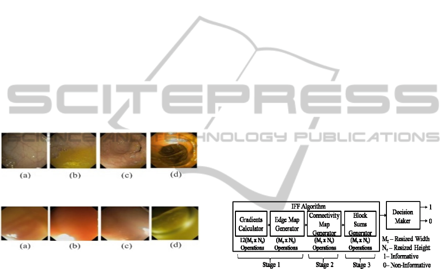
Figure 1: Examples of Informative Frames.
Figure 2: Examples of Non Informative Frames.
As already mentioned, IFF is a fundamental step
for generating quality measurement of colonoscopy
video for both post-processing and real-time. To
provide automated quality measurement in real-time
for colonscopy videos which are captured at 30 fps
(frames per second), we have only around 33 ms
(milliseconds) window to process each frame and
generate quality metrics if all 30 frames are need to
be processed. There are several steps to generate
quality metrics. For a good real-time system, we
ensure that all these steps are completed in that 33ms
time inteval. Therefore, the primary design
consideration of IFF software module is to consume
as less time as possible (below 33 ms), and to leave
the more remaining time for other steps to execute.
The major contributions of this paper can be
summarized as follows: Our previous edge-based
algorithm [Oh, J., et al. 2007] is inaccurate due to
lack of consideration of the deeper meaning of
informative colon frames. We propose a new edge-
based algorithm with higher accuracy compared to
the previous one. IFF is the first among many other
steps in automated colonoscopy quality
measurement. Based on our new algorithm, we
propose a software solution using GPU to evaluate
frame quality under real-time constraints.
2 PROPOSED IFF ALGORITHM
We describe three major requirements for effective
IFF based on our new definition of informative
frame (Section 1) below.
The first requirement is to produce an edge map
which shows connectivity only when there is
"information", and does not show any hints of
connectivity when there is no "information". The
second requirement is to estimate the amount of
connectivity possessed by an edge map, and the third
requirement is to quantify the percentage of
connected pixels. Based on a threshold for the
percentage, we make the final decision whether a
frame is informative or not. Both the second and the
third requirements could not be satisfied using our
previous edge-based technique. We design our new
algorithm by dividing it into three stages based on
these three requirements (Figure 3).
Figure 3: New IFF Algorithm Scheme.
2.1 Stage-1: Generating Edge Map
To satisfy the first requirement, we need an edge
detector which can detect connected edge pixels if
there is any real information. Based on our
experiences, low-sensitivity edge detector is better
for this. So, the fundamental rule of thumb for edge-
based IFF is to use low-sensitive parameters for
edge detection. Despite of low-sensitivity, Canny
edge detector generates vivid lines for non-
informative frames, which may be misinterpreted as
information. We found Sobel edge detector [Canny,
J., 1986] with low-sensitive parameters can be better
than Canny edge detector.
With Sobel edge detector as the choice, we
generate the edge map as follows. If p is a pixel
point at the location (x, y) in a gray scale image, and
q is a pixel point at the same location (x, y) in its
BIOSIGNALS 2011 - International Conference on Bio-inspired Systems and Signal Processing
120
binary edge map, then their values are represented
by f(p) and e(q), respectively. The relationship
between them is defined by the equation: e(q) =
T[f(p)], where T is Sobel operator. The Sobel
operator could be separated into x-direction and y-
direction operators. If the two Sobel operators are
applied to a pixel position, the resulting gradient
could be defined as ∇f = (Gx, Gy). The magnitude of
the gradient is defined as
║∇f ║ = [G
x
2
+ G
y
2
]
1/2
(1)
The range of ║∇f║ varies. To standardize the edge
detection criteria, we approximate this value to a
value between 0 and 1. Hence, if ‘ε’ is defined as a
threshold for Sobel edge detector, the binary edge
map at pixel ‘q’ is given by,
e (q) = 0, if 0 ≤ ║∇f║ ≤ ε, otherwise, e (q) = 1
(2)
To ensure that the low-sensitivity rule of thumb
is satisfied, we chose the threshold value for Sobel
edge detector, ‘ε’ as 0.33.
2.2 Stage-2: Generating
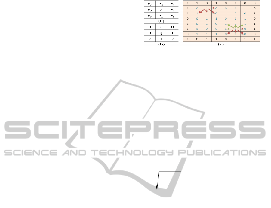
Connectivity Map
In this stage, first, we generate a connectivity map to
estimate the amount of connectivity from an edge
map generated in Stage 1. An edge pixel’s
connectivity, C
x,y
can be described as the amount of
connectivity it possesses with its neighbouring edge
pixels in a 8-connected neighbourhood (Figure 4(a)).
According to the definition of an informative frame
in Section 1, colon frames are considered more
informative (or connected) if there are more
diagonal connections in their edge map. If we give
the same weight to both adjacent (vertical and
horizontal) and diagonal connections, it will not
properly quantify the amount of connectivity for the
IFF. Hence, we give diagonal connection twice the
weight of an adjacent connection.
Second, the connectivity at ‘q’ in edge map is
calculated based on its connection to only four of its
neighbouring pixels (immediate right, immediate
bottom, immediate diagonal left, immediate diagonal
right), and these are shown with red arrows in Figure
4(c)). This is done to avoid redundancy (redundancy
is marked with light green arrows in Figure 4(c)) in
the calculation of cumulative connectivity when
traversing from top left to bottom right corners of
the image. For easier computation of connectivity, a
non-redundant connectivity mask is designed
(Figure 4(b)). In an 8-connected neighbourhood, the
connectivity at pixel 'q', is given by,
C
x
,
y
= (
z
6
+2
z
7
+
z
8
+2
z
9
) * e (q). (3)
Figure 4: (a) 8-connected neighbourhood with 0 ≤ {z
1
,
z
2
… z
9
} ≤ 255 if c=p and 0 ≤ { z
1
, z
2
… z
9
} ≤ 1 if c=q; (b)
Non-redundant connectivity mask; (c) Explanation of
redundancy during connectivity calculation in an edge
map.
2.3 Stage-3: Quantifying the
Informative Portion of a Frame
To quantify the information, the connectivity map is
divided into a number of blocks, and checked for the
number of blocks which have sufficient connectivity
(or information). The image is resized to (M
r
, N
r
),
such that the height and width are multiples of block
size m x m. So, with a block size of m x m pixels, the
total number of blocks will be, µ = (M
r
x N
r
)/(m x
m). The total connectivity of a block, B
i
, is given by,
B
i
=
∑
−−
=
1,1
0,
,
mm
yx
yx
C
, where i = 1, 2, 3…. µ.
(4)
If ‘€’ is defined as the block connectivity
threshold, then a block is considered as non-
informative if B
i
≤ €. Assume that a connectivity
map has β number of informative blocks. If we
define α as the ratio of informative blocks over total
blocks, and ф as a threshold for informative block
ratio, then α = β/µ; a frame is considered informative
if α ≥ ф. After careful experimental analyses on
many frames, the chosen set of parameters is: m =
64, ε = 0.33, € = 5, ф = 0.3. The new algorithm’s
accuracy results are discussed in Section 5.2.
From Figure 3, the computational cost of IFF
algorithm can be 15(M
r
x N
r
) since Stage 1 has
13(M
r
x N
r
), Stage 2 has (M
r
x N
r
), and Stage 3 has
(M
r
x N
r
), which are all numerically intensive
sequential iterations. We mitigate these costs by
using the many-core GPU (Graphics Processing
Unit).
3 GPU ARCHITECTURE
For a GPU, the ‘EVGA 01G-P3-1280-RX GeForce
GTX 280 1GB 512-bit GDDR3 PCI Express 2.0 x16
HDCP Ready SLI Support Video Card’ was used.
This graphics card has 1 GB global memory and 256
EFFECTIVE AND ACCELERATED INFORMATIVE FRAME FILTERING IN COLONOSCOPY VIDEOS USING
GRAPHICS PROCESSING UNIT
121
KB L1 texture cache. From hardware standpoint, the
card is viewed as a combination of 10
Texture/Thread Processing Clusters (TPCs). Each
TPC holds 24 KB L2 texture cache, and evenly
distributes it across three Streaming Multi-
processors (SMs). Each SM has 8 scalar processors
(SPs), 16 KB of shared memory, and 32 KB register
file which is evenly partitioned amongst resident
threads when the device is used for computing. From
programming standpoint, we use the NVIDIA®
CUDA™ (Compute Unified Device Architecture)
programming model [NVIDIA CUDA Programming
Guide 3.0-beta1, 2009] to run this device in
computing mode with CUDA Compute Capability
1.2. CUDA views the device as a pool of threads
and calls it a Grid.
4 IFF ALGORITHM ON GPU
In this section we are implementing the IFF
algorithm discussed in Section 2 on a GPU using
CUDA. We use three types of memories for our
algorithm - Global, Texture and Shared memories.
In Global memory, its size is large (i.e., 1GB as
mentioned in Section 3), but it has more latency
(means less speed) compared to other GPU
memories. When the CUDA threads access data in
global memory with an offset, the speed is further
reduced [CUDA Programming Best Practices Guide
3.0-beta1, 2009] since the data is stored in a linear
pattern (Figure 5(b)). In our GPU implementation,
therefore, global memory is limited to only those
CUDA kernels in which memory access with an
offset is not present.
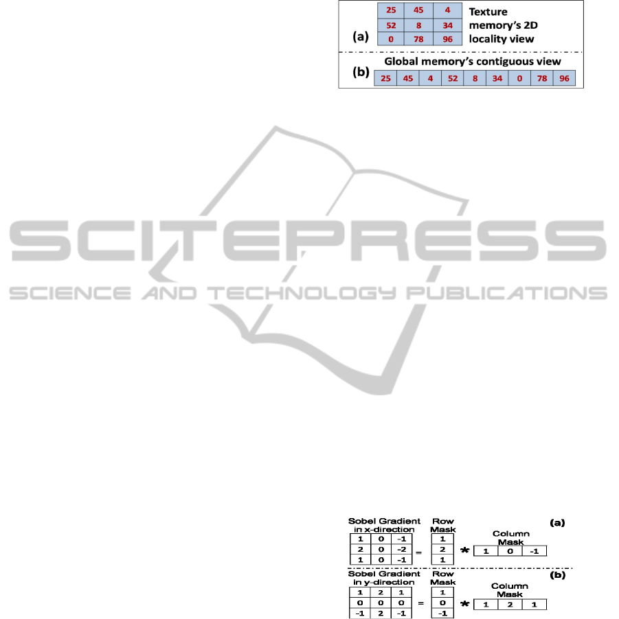
In Texture memory, data is stored in a two-
dimensional pattern (Figure 5(a)). So, when CUDA
threads need to access data with an offset, texture
memory is preferred to global memory for better
speed because it is cached and offset access will be
performed in a symmetric 2-D pattern (Figure 5(a))
rather than linear 1-D pattern as in global memory
(Figure 5(b)). In Shared Memory, the data is stored
on the chip (i.e., the Streaming Multiprocessor
(SM)) in linear pattern. It is faster than global
memory because it is an on-chip memory, but it has
a limited space of 16KB per SM (Section 3). It is
used when the number of threads operating on a data
keeps changing or when threads access the same
data again and again in a loop while performing a
particular operation in a CUDA kernel.
Throughout the GPU implementation, we set the
number of CUDA threads in x-direction as 16 and y-
direction as 8, making it a total of 128 threads per
CUDA thread block. With this background, we
present the GPU implementation of each stage of
IFF algorithm next.
Figure 5: (a) 2-D Locality View of Texture Memory; (b)
Linear or 1-D view of Global Memory.
4.1 GPU Implementation of Stage 1
The input of Stage 1 is a gray scale frame, and the
output is a binary edge map comprising 0's and 1's.
The gray scale image data is copied to global
memory of the GPU. According to Section 2, we
first need the Sobel component gradients in x- and y-
directions. Then, based on Equations (1) and (2), we
evaluate the actual gradient to output an edge map.
We divide the GPU implementation into three steps
here. In Step 1, we calculate the Sobel gradient in x-
direction using separable Sobel masks. An original
Sobel mask has 3x3 dimensions, and it is separable
into 3x1 and 1x3 masks whose product will give us
back the original 3x3 mask (Figure 6(a) and 6(b)).
We call these masks as row mask and column mask
for convenience. We apply row mask to the gray
scale image first and then we apply the column mask
to that result in order to obtain the final Sobel
gradient component in x-direction. We use separable
filters because the offset required to access data is
less and this helps in improving the execution time
of the program.
Figure 6: (a) Separable Masks for Sobel gradient in x-
direction; (b) Separable Masks for Sobel gradient in y-
direction.
In Step 2, we calculate Sobel gradient in y-
direction using another set of separable Sobel masks
in exactly the same way explained before for Sobel
gradient in x-direction. Since texture memory is
read-only, we store the gradients in the global
memory. In Step 3, we compute the edge map based
on Equations (1) and (2). Here, we do not need
BIOSIGNALS 2011 - International Conference on Bio-inspired Systems and Signal Processing
122

texture memory because threads do not access data
with an offset. So, we perform computations of
Equations (1) and (2) using GPU registers and store
the final edge map in global memory. Due to the fact
that we used CUDA threads and blocks with 100%
device occupancy, we will obtain a good speed
despite using global memory here.
4.2 GPU Implementation of Stage 2
The input of Stage 2 is the edge map obtained from
Stage 1. The output is a connectivity map which is
obtained by applying the connectivity mask shown
in Figure 4(b) and Equation (3). As we see in Figure
4(b), connectivity mask is not separable like a Sobel
mask. So, we access the edge map which resides in
global memory via texture memory, then perform
the computations of Equation (3) using registers.
The result (connectivity map) is stored back in
global memory. We do not use shared memory in
either Stage 1 or Stage 2, and limit our calculations
to texture memory because the masks applied in
both stages are of size 3x3 pixels, which is small.
4.3 GPU Implementation of Stage 3
The input of Stage 3 is a connectivity map from
Stage 2. The output is the block sums obtained by
performing computations on the connectivity map
based on Equation (4). In Section 2.3, we choose the
block size as 64 x 64. According to Equation (4), we
are supposed to calculate the square root of sum of
values of all 64 x 64 pixels (i.e., a total of 4096
pixels) for each block in the connectivity map. We
divide this stage into two steps. Initially, the
connectivity map resides in the global memory. We
use 128 threads per CUDA block to perform the sum
of 4096 pixels as follows. In Step 1, we first assign
each thread in a CUDA block to add 4096/128 = 32
pixels in global memory, and store the results in
shared memory. In other words, we have 128
parallel partial sum computations using global
memory. We do not use share memory in this step
because we will loose the 100% device occupancy
and eventually loose speed if we load 4096 pixels
into the shared memory directly just to perform a
simple addition. So, now we have 128 elements in
shared memory for each CUDA block.
In Step 2, we use parallel summation in shared
memory [CUDA Technical Training, 2008]. We
reduce the number of threads to 64 such that each
thread adds two consecutive pixel values and stores
it back in shared memory. Now, we have 64 values
in shared memory. We reduce the number of threads
to 32 and perform the same operation again. This
process is repeated until we get the final sum of
4096 pixels. We perform Step 2 using shared
memory because the number of threads performing
summation is varied at every level of summation,
and these threads repeatedly access same locations.
Utilizing shared memory is more effective than
using global memory in this case. Finally, we obtain
the block sums of each block, and we perform a
square root operation on each block sum (according
to Equation (4)) in shared memory, then transfer the
block sums back to global memory.
Next, we calculate the number of blocks which
are informative based on a threshold and decide
whether a frame is informative (see Section 2.3) on
CPU. This is a trivial operation and does not require
GPU power.
5 EXPERIMENTS AND RESULTS
For our experiments, we used a machine having an
Intel Quad Core CPU @ 3.0 GHz with 3 GB RAM
and an NVIDIA GTX 280 card with 1 GB GDDR3.
For execution time acceleration, we compared our
GPU implementation with CPU-only
implementation. We used C language for CPU-only
implementation. For effectiveness, we compare our
new IFF algorithm with our previous one [Oh, J., et
al. 2007].
5.1 Acceleration
We present a comparative analysis of GPU and CPU
versions of the IFF algorithm on different frame
types (Table 1). We chose six different video input
sources with different frame resolutions, and fed
them to our CPU and GPU IFF algorithm versions.
Each algorithm is run over more than a 100 frames
of every video type. Table 1 shows the average
processing times taken by the CPU/GPU IFF
algorithms to process a single frame belonging to
each of these video inputs.
From Table 1, with the increase in the frame
size, the CPU processing time increases rapidly. On
the other hand, the GPU processing time increases
minimally. When programmed with CUDA for
numerical data intensive operations, the results are
also a testimony of the instruction throughput and
memory throughput achieved by the kernels we
designed for our GPU algorithm. For the highest
resolution frame we tested (HD 1080), we achieved
up to 40x speed- up using our new GPU IFF
algorithm. The commonly used video capture
EFFECTIVE AND ACCELERATED INFORMATIVE FRAME FILTERING IN COLONOSCOPY VIDEOS USING
GRAPHICS PROCESSING UNIT
123

resolution standard currently is DVD, but we are
expecting HD videos to replace the DVD format
soon.
Table 1: IFF Software Module Results for a single frame
from different video inputs.
Video Type Frame Size GPU (ms) CPU (ms) Speed Up
VGA 640 x 480 6.73 85.76 12.74
DVD 720 x 480 8.0 94.46 11.81
HD 576 720 x 576 9.53 121.99 12.8
XGA 1024 x 768 12.7 236.29 18.61
HD 720 1280 x 720 11.58 268.81 23.22
HD1080 1920x 1080 14.88 595.12 40.0
5.2 Effectiveness
We use typical four quality metrics (Precision,
Sensitivity, Specificity and Accuracy) shown to
evaluate the performance of the new and the
previous algorithms. The ground truths of the
informative and the non-informative frames were
verified by the domain expert. Table 2 shows the
average values for 10 colonoscopy videos. Table 2
shows that our new algorithm discussed in this paper
(IFF#2) outperforms our previous algorithm [Oh, J.,
et al. 2007] (IFF#1) in all four metrics. IFF#2
provided around 97.6% of accuracy – meaning 7%
increase compared to our previous one – IFF#1
which offers only 90.6 accuracy for this data set. We
tested more than 100 videos, and found that our new
algorithm has around 96% overall accuracy.
Table 2: Comparison of Previous (IFF#1) and New
(IFF#2) algorithms on over 100 videos.
Metrics IFF#1 IFF#2
Precision 89.1% 97.0%
Sensitivity 88.3% 97.9%
Specificity 92.1% 97.0%
Accuracy 90.6% 97.6%
6 CONCLUSIONS
In this paper, we discussed a new IFF algorithm
which is around 15% more accurate compared to our
previous algorithm. Through a proper understanding
of the meaning of an informative frame, we
introduced a new definition to an informative colon
frame. The computing constraints which reside
within the algorithm have been mitigated with our
IFF software module which consumes 8 ms
(Table 1) out of the total real-time constraint – 33
ms (Section 1), and provides 25 ms credit for other
steps of automated colonoscopy quality
measurement to complete. In comparison to CPU,
our GPU algorithm is 40 times faster for a HD 1080
video. Our future work will be focused on
combining multiple GPUs together to further
accelerate colonoscopy video analysis.
ACKNOWLEDGEMENTS
This work is partially supported by NSF STTR-
Grant No. 0740596, 0956847, National Institute of
Diabetes and Digestive and Kidney Diseases
(NIDDK DK083745) and the Mayo Clinic. Any
opinions, findings, conclusions, or recommendations
expressed in this paper are those of authors. They do
not necessarily reflect the views of the funding
agencies. Johnny Wong, Wallapak Tavanapong and
JungHwan Oh hold positions at EndoMetric
Corporation, Ames, IA 50014, U.S.A, a for profit
company that markets endoscopy-related software.
Johnny Wong, Wallapak Tavanapong, JungHwan
Oh, Piet de Groen, and Mayo Clinic own stocks in
EndoMetric. Piet de Groen, Johnny Wong, Wallapak
Tavanapong, and JungHwan Oh have received
royalty payments from EndoMetric.
REFERENCES
American Cancer Society, 2008. “Colorectal Cancer Facts
and Figures” http://www.cancer.org/docroot/
STT/content/STT_1x_Cancer_Facts_and_Figures_200
8.asp.
Johnson, D., Fletcher, J., MacCarty, R., et al. 2007.
“Effect of slice thickness and primary 2D versus 3D
virtual dissection on colorectal lesion detection at CT
colonography in 452 asymptomatic adults”, American
Journal of Roentgenology, 189(3):672-80.
Pabby, A., Schoen, R., Weissfeld, J., Burt, R., Kikendall,
J., Lance, P., Lanza, E., Schatzkin, A., 2005.
“Analysis of colorectal cancer occurrence during
surveillance colonoscopy in the dietary prevention
trial". Gastrointestinal Endoscopy, 61(3): p.385-391.
Oh, J., Hwang, S., Lee, J., Tavanapong, W., de Groen, P.,
Wong, J., 2007. “Informative Frame Classification for
Endoscopy Video”. J. Medical Image Analysis,
11(2):110-27.
Canny, J., 1986. “A Computational Approach to Edge
Detection". IEEE Trans. Pattern Analysis and
Machine Intelligence, 8:679-698.
NVIDIA CUDA Programming Guide 3.0-beta1, 2009.
www.nvidia.com.
CUDA Programming Best Practices Guide 3.0-beta1,
2009. www.nvidia.com.
CUDA Technical Training, 2008. Vol. I: Introduction to
CUDA Programming, www.nvidia.com.
BIOSIGNALS 2011 - International Conference on Bio-inspired Systems and Signal Processing
124
