A COLLECTIVE BIOLOGICAL PROCESSING ALGORITHM

FOR ECG SIGNALS

Horia Mihail Teodorescu

FAS, Harvard University, Cambridge, MA, U.S.A.

Keywords:

Swarm model, Signal processing, Filtering, Biologic signal, EKG.

Abstract:

We establish and explore an analogy between hunting by packs of agents and signal processing. We present a

version of adaptive ‘Hunting Swarm’ algorithm (HSA), apply it to ECG signals, and investigate the inﬂuence

of the model parameters on the ﬁltering of stationary and nonstationary noise. We show that results obtained

with the HSA ﬁlter may outperform results obtained with several other ﬁlters.

1 INTRODUCTION

Biological signals have wide bandwidth and may be

affected by various noises. The ﬁrst stage in process-

ing such signals consists of ﬁltering them in order

to achieve a good signal to noise ratio (SNR). This

task is often challenging because of the wide band of

the signals and of the noises. As a consequence, nu-

merous papers have been published recently propos-

ing new ﬁltering methods for ECG signals (Almenar

and Albiol, 1999), (Leski and Henzel, 2005), (Ko-

tas, 2007), (Korrek and Nizam, 2010), (Bansal et al.,

2009), (Yan et al., 2010).

In a previous communication (Teodorescu and

Malan, 2010), we introduced an image processing al-

gorithm based on swarms. In this paper we explore

several variants of the ‘hunting swarm algorithm’

(HSA) and analyze their ability to remove noise from

EKG signals for various signal to noise ratios (SNR).

The signal is ‘enacted’ by the trajectory of a prey

hunted by the swarm, as detailed in section 2.

The models of the swarms in this paper include

salient features from various swarm models reported

in the literature and features that we introduced based

on general considerations or from experimentation

with model parameters.

The organization of the paper is as follows. In the

second section we expose the method to transform the

signal processing task into a pack-hunting-a-prey task

and describe the equations describing the prey and the

pack movements. The third section is devoted to the

results of ﬁltering ECG signals with the HSA algo-

rithm. The details of the implementation and the re-

sults are discussed in the fourth section. Conclusions

are drawn in the last section.

2 THE HS SIGNAL PROCESSING

METHOD

2.1 Metaphor of the Hunting Pack

In this section we suggest and exploit an analogy be-

tween signal ﬁltering and the natural hunting packs.

We use this analogy to produce an algorithm for non-

linear signal processing. The analogy has two main

players: the prey and the hunting pack. The prey does

not collaborate to the signal processing; instead, it en-

acts the signal. The pack performs a virtual hunting

and in so doing it produces the output (processed) sig-

nal as the trajectory of the center of the pack. The

hunting pack model, while borrowing much from var-

ious swarm models, has many new features that give

reason to consider it a new swarm model.

Figure 1 depicts a sketch of a simpliﬁed process-

ing procedure. In this sketch, the swarm is assumed

constrained on a line at each time moment, with the

agents taking positions along that vertical line, ac-

cording to movement equations governed by inter-

agent forces and to agent to prey forces. The prey

moves in discrete time along the signal. The agents

are attracted by the prey, thus tending to follow the

prey. Consequently, the center of the swarm describes

a trajectory in the plane. That trajectory is the result

of ‘processing’ the prey trajectory, i.e. the signal, by

the swarm.

413

Mihail Teodorescu H..

A COLLECTIVE BIOLOGICAL PROCESSING ALGORITHM FOR ECG SIGNALS.

DOI: 10.5220/0003136304130420

In Proceedings of the International Conference on Bio-inspired Systems and Signal Processing (BIOSIGNALS-2011), pages 413-420

ISBN: 978-989-8425-35-5

 2011 SCITEPRESS (Science and Technology Publications, Lda.)

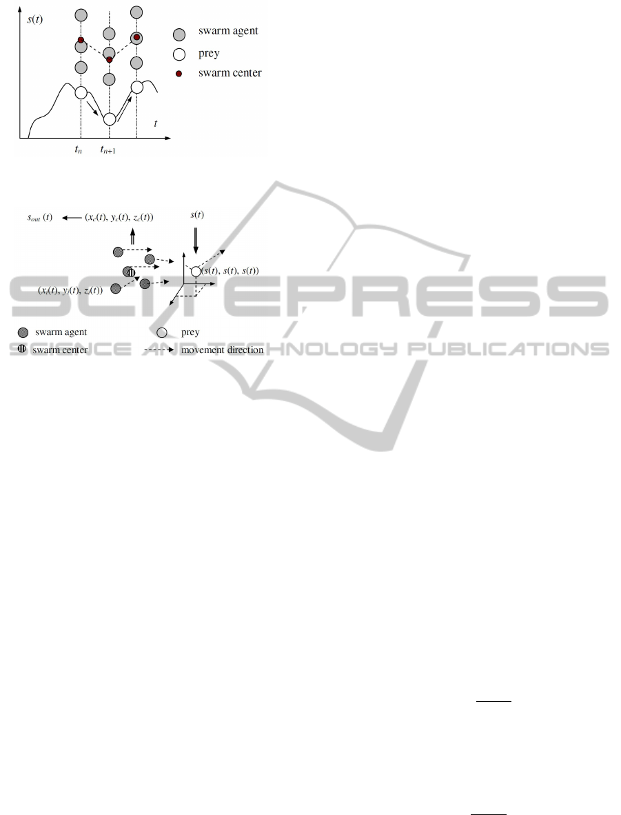
Figure 1: Sketch of the operation of the swarm as signal

processing system.

Figure 2: Sketch of the operation of the swarm as signal

processing system.

Figure 2 shows a sketch of the procedure in three

dimensional (3D) space. In this sketch, the prey

moves along a trajectory represented by (x

(t) =

s(t),y

(t) = s(t),z

(t) = s(t)) and represents the in-

put signal marked by the double line arrow in the up-

per right side of the ﬁgure, while the center of the

pack represents the output signal.

The use of this metaphor in signal de-noising

is based on the hypothesis that hunting swarms are

able to ﬁlter out ‘undue’, ‘evasive’, that is, noise-like

changes in the trajectory of the prey during the hunt-

ing. Moreover, swarms might use a simple collective

adaptation of its behavior to closely follow the prey

when the last had the chance to take a larger distance.

These hypotheses were veriﬁed during simulations, as

demonstrated by the result section. The consequence

is the present proposal of HS ﬁltering method.

Because the model is somewhat elaborate, we in-

troduce in the subsequent section the equations of the

swarm, neglecting the prey, while in the 2.3 subsec-

tion we take into account the prey inﬂuence and the

adaptive behavior of the prey as elicited by the prey

movement.

2.2 Swarm Basic Equations

Hunting takes place according to a set of equations

that govern the movements of the agents in the pack.

These equations have three types of components. The

ﬁrst type comprises ‘physical’ forces like the inertia

and the friction forces. The second class of forces

includes the interaction forces inside the pack; these

forces keep the pack together, while preventing agents

from colliding one with the other. The agents are

endowed with an elementary memory and with an

awareness to the global state of the pack, moving

accordingly. Finally, the ‘external’ force that pro-

duces the movement of the swarm is the interaction

of the agents with the hunted prey. The general equa-

tion governing a swarm is, according to (Reza Olfati-

Saber and Murray, 2007):

˙x

(t) =

∑

j∈N

(t) − x

(t)) + b

(t) (1)

with the initial conditions x

(0) = z

and b

(t) = 0.

Above, x is a spatial coordinate, i, j denote agents of

the swarm, b is due to an external force (bias). The

left hand side of the equation represents the velocity,

while the terms under the sum in the right-hand side

are similar to elastic forces, F = κ · (x

− x), where κ

is the elastic constant and x

is a ﬁxed position. For

the swarm, x stands for the position of the agent x

and x

is replaced by that of the prey, x

. In case of

consensus algorithms, the above equation in discrete

time and without the term b

is (Reza Olfati-Saber and

Murray, 2007):

[t + 1] = x

[t] + ct ·

∑

j∈N

i j

· (x

[t] − x

[t]) (2)

where a

i j

are constants and t denotes here a discrete

time moment. Under certain conditions, the swarm is

stable, which in terms of consensus theory means that

a consensus is asymptotically reached (Reza Olfati-

Saber and Murray, 2007).

Kim (Kim, 2008) used artiﬁcial potential func-

tions to model the attraction towards the goal. We use

a similar approach, but with different potential func-

tions, moreover also including repulsive forces that

replace the attractive ones starting with a given dis-

tance. The potential forces we use have the form:

(i) - for the repulsive forces:

i, j

= −k

− x

i, j

(3)

for d

i, j

≤ ρ

, where k

is a positive constant, d

i, j

is the

distance between the agents denoted by the indices i

and j, η

is a natural power, and ρ

is a constant;

(ii) - for the attractive forces:

i, j

= k

− x

i, j

(4)

for d

i, j

≤ ρ

, where k

is a positive constant, d

i, j

is the

distance between the agents denoted by the indices i

BIOSIGNALS 2011 - International Conference on Bio-inspired Systems and Signal Processing

414

and j, η

is a natural power, and ρ

> ρ

is a constant.

The constants in the above equations are parameters

of the processing system.

The above forces create accelerations that are

computed as:

u,i

[t + 1] = −k

∑

[t − 1] − u

[t − 1]

i, j

[t − 1]

(5)

where u stands for x, y, or z and a

u,i

is the acceler-

ation in the direction u of the agent i due to the re-

pulsion at small distances from the other agents in the

pack, or due to attraction at larger distances. Sub-

sequently, we use the ﬁrst order approximations of

the derivative, ˙u[t] = (u[t] − u[t − 1]) · δ, where u is

a coordinate variable, t is a discrete variable stand-

ing for time, and δ is the step for time discretiza-

tion. Then, the inertial force along the u direction

is m · ¨u = m · (v

[t] − v

[t − 1]), where v

is the ve-

locity along the u direction and m is the mass, which

we assume unitary for all agents in the pack. Based

on the acceleration, according to the last equation, the

change of velocity is computed as

u,i

[t + 1] = v

u,i

[t] + δ · a

u,i

[t]. (6)

In (6), δ is the time step interval and represents an

important parameter in the simulations. Larger values

of δ make the pack respond faster to the signal, but

can produce overshoots when the signal varies fast.

We used values of δ between 0.5 and 2 for best results.

Next, we include in equation 6 the effect of fric-

tion forces, that we assume to have components

proportional to the respective velocity component,

u, f riction

= µ · v

. The change in velocity due to the

friction is ∆v

= F

u, f riction

÷ m = −ct. · v

, where the

constant includes µ, the time step, δ, and the inverse of

the mass, m

−1

. For ease of writing, subsequently we

denote by µ the constant in the change of the velocity

due to friction, ∆v

[t + 1] = −µ · v

[t].

2.3 Prey Inﬂuence and Adaptive

Swarms

The prey is assumed to move independently of the

movement of the hunting swarm. This hypothesis is

unsuitable for biological or physical modeling pur-

poses, but it is required by the task we deal with, be-

cause the signal, enacted by the prey, should remain

independent of the processing. On the other side, the

prey ‘attracts’ the hunting swarm. The attraction force

we use is a third order, nonlinear, elastic-type force

with the expression:

u;a,p

= A

· (u

− u

) + A

· (u

− u

)

≥ 0

(7)

where u

are the coordinates of the prey and A

, A

are model constants. Including the contribution of the

prey to the acceleration of the agents, the equation (6)

rewrites

u,i

[t + 1] = v

u,i

[t]+ (8)

+δ · a

u,i

[t] + A

· (u

− u

) + A

· (u

− u

)

. (9)

where, again, we assume that we included the δ fac-

tor in the constants A

without changing the nota-

tions. The position of the agent at time step t + 1 is

obtained as

[t + 1] = u

[t] + δ · v

u,i

[t]. (10)

A set of restrictions, like a limit in acceleration and

a limit in the change of direction are added, which

have intuitive biological counterparts. We skip details

here, but we used these limits in the swarm processing

system whose results we describe.

Once the positions of the N swarm agents at time t

are computed, we determine the position of the center

of the swarm as

[t] =

∑

[t]. (11)

It is natural at the biological level that agents in

the swarm are aware of the behavior of the swarm as

a group and to adjust to it. We make a further hy-

pothesis, that in a hunting pack the agents are aware

of the relative position of the pack and the prey, ad-

justing their speed according to that relative position.

Namely, we assume that, whenever the distance from

the center of the pack to the prey becomes too large,

every agent will increase its velocity by a factor pro-

portional to u

− u

. So, if |u

− u

| ≥ D, an in-

crease in velocity ∆v

u,i

= B · (u

− u

) occurs for all

the agents. This conditional increase of the agents

velocity stands for an elementary adaptation to the

momentary conditions of hunting. From the point of

view of the HS ﬁltering algorithm, this adaptive be-

havior means better results in case the signal has fast

transients or fronts. We skip technical details related

to the algorithm implementation and provide some of

them in the Appendix.

The choice of the forces governing the swarm

behavior was made based on considerations related

to the dynamic bahavior. These considerations are

quite transparent and intuitive at the physical level.

For example, the use of the third order, nonlinear,

elastic-type force increases the speed of reaction of

the swarm to fast changes in the signal, while the use

of limits in acceleration and limits in the change of

direction of the agents insures that the agents and the

swarm have limited overshoots. The use of odd pow-

ers in the forces expressions are also rationally moti-

vated: even powers loose the direction information in

the relative positions of the agents and the prey.

A COLLECTIVE BIOLOGICAL PROCESSING ALGORITHM FOR ECG SIGNALS

415

3 PROCESSING RESULTS

We exemplify the results we obtained with the HS

signal processing method applied to EKG signals.

We used the signal database PhysioBank (Goldberger

et al., e 13). All input signal ﬁlenames referred to

in the ﬁgures are from Physiobank, to which we add

noise. We show two categories of results. The ﬁrst

one refers to noisy EKG from the cited database; the

second refers to ﬁltering results obtained when apply-

ing the processing to relatively clean EKG signals that

we corrupted with uniform noise of various ampli-

tudes. Notice that the noisy ECG signals include true

noise; to these we have not added any extra noise.

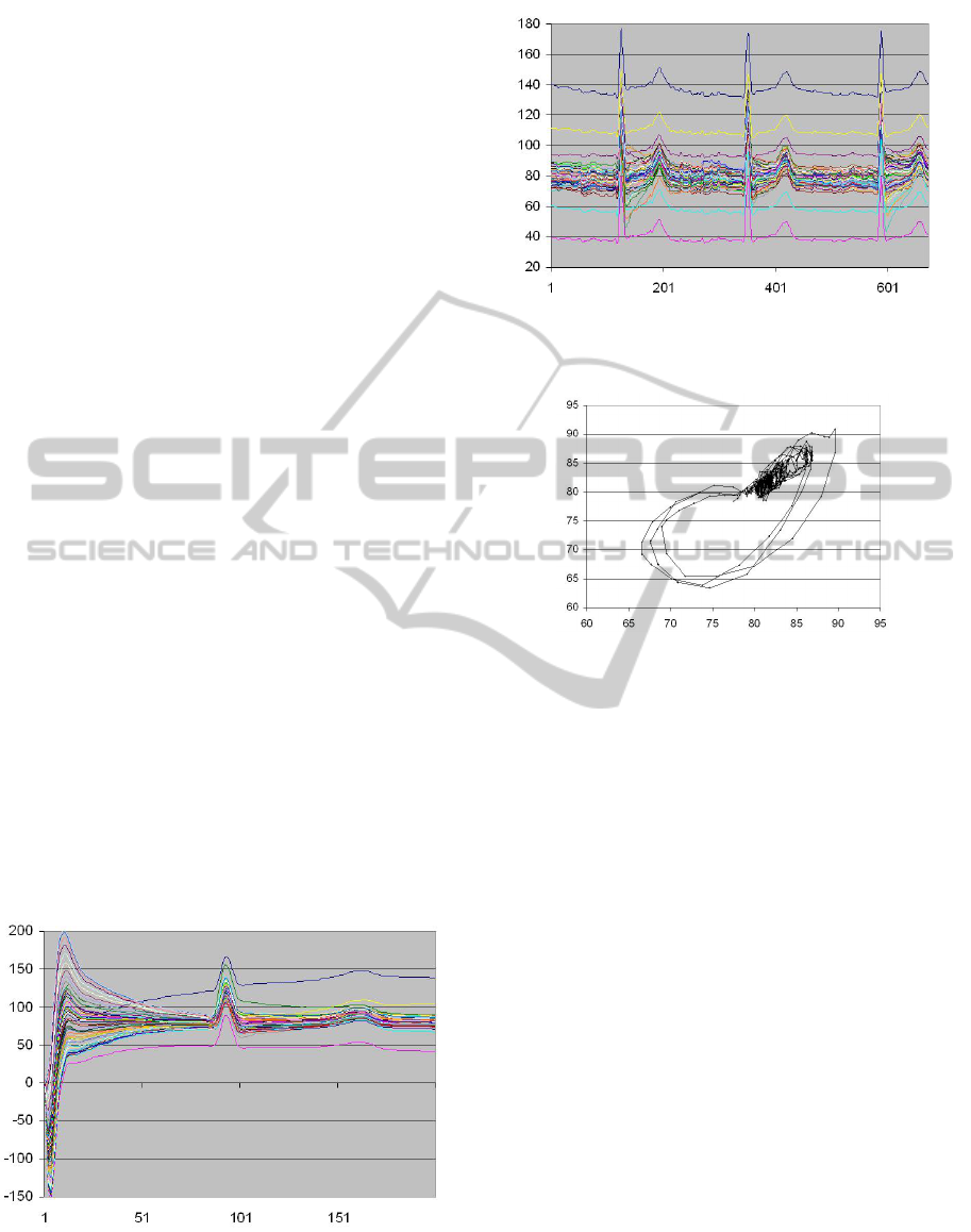
3.1 Mechanics of the Filtering Process

The mechanics of the HS processing is revealed by

the representation of the trajectories of all the agents

in the pack and by a representation of the dependency

of the evolution of the center of the pack with respect

to the processed signal. The ‘hunting’ process has two

phases. In the ﬁrst phase, the pack, which is assumed

to start from random initial conditions, is structuring

itself and evolves toward an almost stable conﬁgura-

tion. This transitory regime is shown in Fig. 3 and

may last about 100 time steps, its duration primarily

depending on the initial positions and on the friction

forces. After the transitory behavior, the swarm re-

mains almost stable, despite its continuous movement

driven by the prey. Only when the signal has very

fast variations, the swarm may be partly de-structured

and needs some time to recover its equilibrium. This

regime of dynamic stability is shown in Fig. 4 for a

swarm including 55 agents.

Figure 3: Transitory regime of the hunting pack takes about

100 time steps for this swarm of 55 agents, with µ = 0.35,

= η

= 4.

Figure 4: Processing result with a swarm with 55 agents,

using the fourth power of distances in the inter-agent repul-

sive and attraction forces and a friction coefﬁcient µ = 0.35.

Figure 5: Swarm trajectory plot versus the signal.

The representation of the trajectory of the center

of the swarm as an implicit function of the trajectory

of the prey shows, for almost all processed signals,

that two or three regimes occur during the ‘hunting’,

regimes that are represented by the loops in the dia-

gram in Fig. 5.

3.2 Filtering Noisy Signals

For determining the usefulness of HS ﬁltering, we

tested the swarm ﬁlters with signals from the bench-

mark database PhysioBank ATM (Goldberger et al.,

e 13). Two types of tests were carried on: (i) ﬁlter-

ing signals from PhysioBank that are (intrinsically)

noisy, and (ii) ﬁltering clean signals to which con-

trolled noise is added. The ﬁrst type of tests is needed

for determining if the new ﬁlters are able to solve a

real-life problem; the second type of tests allows us

to investigate the capabilities of the ﬁltering proce-

dure under various controlled conditions.

We exemplify the ﬁltering of noisy signals from

PhysioBank ATM with the signals Fantasia f1y07 and

Apneea ECG A01.

The trajectories of the agents of a swarm of 55

agents during the ‘hunting’ process (Figure 4) are av-

eraged to obtain the center of the pack trajectory. Re-

sults of the HS ﬁltering are shown in Figures .

BIOSIGNALS 2011 - International Conference on Bio-inspired Systems and Signal Processing

416

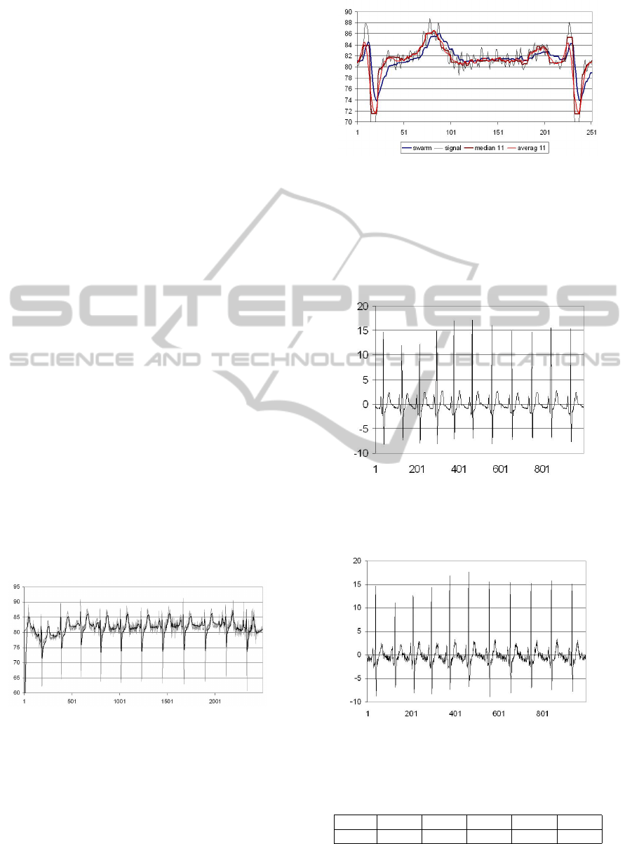
Figure 6: Processing result with a swarm with 55 agents,

using the fourth power of distances in the inter-agent repul-

sive and attraction forces and a friction coefﬁcient µ = 0.35.

Figure 7: µ = 0.35 Original signal and HS ﬁltering result

with a swarm with parameters described in the text.

Figure 8: Detail from the above ﬁgure (µ = 0.65).

The various parameters of the swarm inﬂuence the

results. For example, as expected, a too large fric-

tion coefﬁcient would produce a slower ‘catching’ of

the signal when the signal has large swings, like the

QRS complex. However, the slowing down is not the

same on the upper and lower front of the impulsive

signal, because of the nonlinearity in the swarm be-

havior. This is seen in Fig. 3.

The HS ﬁlters are causal, meaning that they take

into account only previous values of the signal to gen-

erate the current value of the ﬁltered signal. As a con-

sequence, there is a delay between the produced out-

put value and the current value of the signal. For the

numerical evaluation of the performance of the HS

ﬁlters, for example for applying the mean square er-

ror criterion, we need to determine the lag of the ﬁl-

ter. We determined the corresponding lag for a ﬁlter

with speciﬁed parameters minimizing the MSE be-

tween the signal and the HS output, for signals not

Figure 9: The same signal ﬁltered with a swarm with fric-

tion coefﬁcient µ = 0.65.

corrupted with noise, according to the formula:

τ = min

(

∑

t=t

[t + k] − s

[t])

) (12)

where t

are the limits of the interval of determi-

nation (we used t

= 200,t

= 950), s

is the output

signal, and s

the input signal. The results for such

a ﬁlter are given in Table 1, showing that the lag of

this ﬁlter is τ = 3. We removed the lag when we com-

puted the MSE for the ﬁltering of noisy ECGs. Notice

that the lag is variable and can not be predicted be-

forehand. Therefore, using a non-causal swarm ﬁlter

would not solve the lag problem completely. How-

ever, the occurrence of the lag does not inﬂuence the

quality of the ﬁltering. It only affects the manner of

computing the MSE value, which is a secondary is-

sue.

Table 1: MSE errors of the swarm ﬁlter, for various adjust-

ments of the lag. Signal Apnea ECG A01.

delay τ = 0 τ = 3 τ = 5 τ = 6

Total error 6247.8 2624.1 5971.8 7597.9

MSE 2.886 1.870 2.822 3.183

Table 2: MSE errors of the swarm ﬁlter (delay τ = 3), av-

erage and median ﬁlters for the same signal and noise, for

various adjustments of the lag. Signal Apnea ECG A01.

Filter HS τ = 3 average median

MSE 1.870 2.467 2.621

For quantitatively comparing the results of the HS

ﬁlter with the results of median and average ﬁlters,

we run the program over signals corrupted by us with

uniform noise. The same input signal with the added

noise was then ﬁltered with an average ﬁlter and with

a median ﬁlter, both of them with window width of

length 11, centered on the current sample. When the

noise is high, the HS ﬁlter outperforms in terms of

MSE the other ﬁlters, as shown in Table 2.

A COLLECTIVE BIOLOGICAL PROCESSING ALGORITHM FOR ECG SIGNALS

417

4 DISCUSSION

The HS processing method is highly nonlinear and

hence sensitive to the amplitude of the signals. Good

results are obtained with the parameters we used for

signal amplitudes in the ranges seen in the ﬁgures. We

multiplied all signals in the cited database by a factor

of 10 before processing.

The HS ﬁlters are causal and the processing results

have a lag with respect to the signal. To determine the

lag, we shifted the result and compared the sum of

squared errors obtained for various shifts. The lowest

error was obtained, in case of the signal Apnea-ECG

A01 (length 10 seconds, data format: standard) for a

lag of 3 time steps. The total squared error was com-

puted for the various ﬁlters for 750 samples, for the

samples from 200 to 950. We skipped the ﬁrst 200

samples to avoid the transitory regime of the swarm

ﬁlter. The mean square error, MSE, was determined

as MSE

= (

∑

t=200..950

[t] − s

[t])

)/750. The re-

sults related to the determination of the lag are shown

in Table 1 in the Annex.

While the algorithm is O(n) in the number of input

signal samples, the calculations at each step involve

looping over the swarm, moreover involve many mul-

tiplications. As a result, the processing is time con-

suming. A swarm of 55 agents, with η

= 4 and

eta

= 4, implemented in a C++ unoptimized program

that also writes more that 10 ﬁles on the disk, takes

about 3 seconds to process 2500 samples of input sig-

nal. This means that the process can be performed in

real time for ECG signals at a sampling frequency of

about 800 Hz.

The HS ﬁlter produces smoother output than the

average and median ﬁlters of order 11 (see Appendix).

The results are not exactly the same when the code

is run several times. The method is not perfectly de-

terministic, as the swarm starts with random condi-

tions, moreover several conﬁgurations of the swarm

may have the same or similar internal energy, thus al-

lowing the swarm to follow close but not identical tra-

jectories when following the same prey.

The system is not guaranteed stable. For example,

swarms with 25 agents or with 85 agents, the other

parameters being the same as above, are unstable. As

far as the swarm remains stable, the number of agents

in the swarm was found to have less inﬂuence on the

ﬁltering error than parameters like µ and constants in

adaptation.

While we used the analogy with the hunting pro-

cess, the presented algorithm might be regarded as a

social process of agreement of a group with a model,

represented by the signal. While the analogy is simi-

lar with the one of swarms with leaders, it is still diff-

erent, because the leaders are assumed to be inﬂu-

enced by the rest of the group, while the model acts

independently from the behavior of the ‘followers’

group.

5 CONCLUSIONS

The HSA is essentially a new nonlinear ﬁltering algo-

rithm derived as a combination of several approaches

in the literature and with a method of mapping the

signal ﬁltering process into a swarm dynamics. The

HSA ﬁltering was demonstrated on a set of bench-

mark ECG signals with intrinsic and added noises.

The results were compared with those obtained with

the average and median ﬁlters.

The hunting swarm method may work remarkably

well when the parameters of the swarm are trimmed

according to the processed signal and noise peculiari-

ties. However, the trimming procedure is not enough

transparent at this stage of development and the use

of genetic algorithms or other evolutionary method to

improve the behavior of the swarm is desirable. The

main advantage is that the HS ﬁlters leave the signals

that have fast as well as slowly varying regions only

slightly altered, while removing a consistent part of

the noise. In this respect, we found that the HS ﬁlters

behave better than the basic average and median ﬁlters

and combinations of them. We conclude that the HSA

might be a strong candidate in ﬁltering signals with

non-stationary, wide bandwidth noise, where simpler

ﬁlters can not cope. Further research is needed to ex-

tensively compare the swarm-based ﬁlters with other

types of nonlinear ﬁlters.

ACKNOWLEDGEMENTS

I thank Dr. David Malan and Professor Leslie Valiant

for essential advice and critics. Also, I thank the two

anonymous referees for very useful comments.

REFERENCES

Almenar, V. and Albiol, A. (1999). A new adaptive scheme

for e.c.g. enhancement. Signal Processing, 75(3):253

– 263.

Bansal, D., Khan, M., and Salhan, A. K. (2009). A com-

puter based wireless system for online acquisition,

monitoring and digital processing of ecg waveforms.

Computers in Biology and Medicine, 39(4):361 – 367.

Goldberger, A. L., Amaral, L. A. N., Glass, L., Hausdorff,

J. M., Ivanov, P. C., Mark, R. G., Mietus, J. E., Moody,

BIOSIGNALS 2011 - International Conference on Bio-inspired Systems and Signal Processing

418

G. B., Peng, C.-K., and Stanley, H. E. (2000 (June

13)). PhysioBank, PhysioToolkit, and PhysioNet:

Components of a new research resource for com-

plex physiologic signals. Circulation, 101(23):e215–

e220. Circulation Electronic Pages: http://

circ.ahajournals.org/cgi/content/full/101/23/e215.

Kim, D. H. (2008). Self-organization of swarm systems

by association. International Journal of Control, Au-

tomation, and Systems, 6(2):253–262. April 2008.

Korrek, M. and Nizam, A. (2010). Clustering m.i.t.-b.i.h. ar-

rhythmias with ant colony optimization using time do-

main and p.c.a. compressed wavelet coefﬁcients. Dig-

ital Signal Processing, 20(4):1050 – 1060.

Kotas, M. (2007). Projective ﬁltering of time-aligned

ecg beats for repolarization duration measurement.

Computer Methods and Programs in Biomedicine,

85(2):115 – 123.

Leski, J. M. and Henzel, N. (2005). Ecg baseline wander

and powerline interference reduction using nonlinear

ﬁlter bank. Signal Processing, 85(4):781 – 793.

Reza Olfati-Saber, J. A. F. and Murray, R. M. (2007). Con-

sensus and cooperation in networked multi-agent sys-

tems. Proceedings of the IEEE, 95(1):215–233.

Teodorescu, H. and Malan, D. (2010). Image re-morphing,

noise removal and feature extraction with swarm al-

gorithm (poster). Mathematical Methods in Systems

Biology, Israel, Jan. 2010.

Yan, J., Lu, Y., Liu, J., Wu, X., and Xu, Y. (2010). Self-

adaptive model-based ecg denoising using features ex-

tracted by mean shift algorithm. Biomedical Signal

Processing and Control, 5(2):103 – 113.

APPENDIX

In the appendix we present a few more graphical re-

sults of ﬁltering, with details.

Figure 10: Result for the signal Fantasia f1o03 with a AHS

with η

= 3, η

= 4, µ = 0.75,η

= 3,η

= 4.

Comparison of swarm ﬁlter, average ﬁlter and me-

dian ﬁlter. The parameters of the swarm are: Nmax =

55, number of time steps N

Timesteps

= 1001, δ = 1.20,

γ = 0.850,zeta = 3.89, phi

max

= 0.785398, friction

coefﬁcient µ = 0.250, ampliﬁcation inter-agent A =

2.40, ampliﬁcation prey-agent AA = 0.80, ampliﬁca-

tion prey-agent second order term AB = 0.000020,

ampliﬁcation prey-agent AC = 0.60, ampliﬁcation

Figure 11: Comparison of median, average and swarm ﬁl-

ters. The swarm produces a slightly smoother signal. Signal

Fantasia f1o03, η

= 3, η

= 4, µ = 0.75.

adaptive center swarm C = 1.30, adaptation distance

D = 1.20, Noise amplitude Anoise = 0.0005.

The average, median and swarm ﬁlters have been

applied with rectangular windows.

Figure 12: Comparison of median, average and swarm ﬁl-

ters. The swarm produces a slightly smoother signal. Sig-

nal Apnea ECH A01 (µ = 0.25, η

= 3, η

= 4, noise factor

0.0005.

Figure 13: Noisy signal Apnea ECG A01, noise factor

00005.

Table 3: MSE errors of the swarm ﬁlter (delay τ = 3), for

various values of the friction coefﬁcient. Signal Apnea ECG

A01.

µ 0.15 0.20 0.25 0.30 0.35

MSE 2.213 1.944 1.870 1.935 2.009

The next ﬁgure shows details of AHS ﬁltering the

signal Fantasia 1o03.

A COLLECTIVE BIOLOGICAL PROCESSING ALGORITHM FOR ECG SIGNALS

419

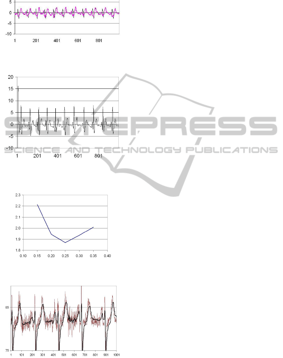
Figure 14: Average and median ﬁlters, window of 11 sam-

ples, centered. Signal Apnea ECG A01, noise factor 00005.

Figure 15: Result of ﬁltering the signal Apnea ECG A01

with the parameters µ = 0.25, η

= 3, η

= 4 for noise

0.0005.

Figure 16: Variation of MSE as a function of the friction

coefﬁcient µ. Signal Apnea ECG A01.

Figure 17: details of AHS ﬁltering the signal Fantasia 1o03.

Friction coefﬁcient µ = 0.75.

BIOSIGNALS 2011 - International Conference on Bio-inspired Systems and Signal Processing

420