A LEARNING APPROACH TO IDENTIFICATION OF
NONLINEAR PHYSIOLOGICAL SYSTEMS USING
WIENER MODELS
Xingjian Jing
Department of Mechanical Engineering, Hong Kong Polytechnic University, Hong Kong
Natalia Angarita-Jaimes, David Simpson, Robert Allen
Institute of Sound and Vibration Research, University of Southampton, Southampton, U.K.
Philip Newland
School of Biological Sciences, University of Southampton, Southampton, U.K.
Keywords: Wiener models, Neuronal modelling, Noninvertible nonlinearity, Noisy data, Lyapunov stability.
Abstract: The Wiener model is a natural description of many physiological systems. Although there have been a
number of algorithms proposed for the identification of Wiener models, most of the existing approaches
were developed under some restrictive assumptions of the system such as a white noise input, part or full
invertibility of the nonlinearity, or known nonlinearity. In this study a new recursive algorithm based on
Lyapunov stability theory is presented for the identification of Wiener systems with unknown and
noninvertible nonlinearity and noisy data. The new algorithm can guarantee global convergence of the
estimation error to a small region around zero and is as easy to implement as the well-known back
propagation algorithm. Theoretical analysis and example studies show the effectiveness and advantages of
the proposed method compared with the earlier approaches.
1 INTRODUCTION
Numerous approaches have been proposed for the
identification of nonlinear systems including
parametric and nonparametric methods (Greblicki
1997, Nelles 2001). Among these, the so-called
block-oriented models have been found very useful
in practice, due to their simplicity in structure and
relative ease of implementation and interpretation.
One of the block-oriented structures is known as the
Wiener model, which consists of a cascade
connection of a linear time invariant (LTI) system
followed by a static (memoryless) nonlinearity. Such
a structure has been shown to be a reasonable model
for many chemical and biological processes (e.g.:
Hunter and Korenberg 1986), as well as
communication and control systems (Huang 1998,
Bloemen et al 2001). Theoretically, any nonlinear
system that has a Volterra or Wiener functional
expansion can be represented (with a sufficient
degree of accuracy) by a finite sum of Wiener
models (Boyd and Chua 1985).
Several different algorithms have been presented
in the literature for the identification of Wiener
models. Early approaches used correlation analysis,
but long periods of data and white Gaussian noise
inputs are required (Billings and Fakhouri 1978).
Approaches based on the invertibility of the static
nonlinearity, and estimation of the linear and
nonlinear blocks either in a successive (Narendra et
al 1966) and iterative procedure or in a simultaneous
manner (Gomez and Baeyens 2004, Kalafatis 1997)
have also been proposed. The main disadvantage of
such algorithms is that convergence is difficult to
guarantee. Moreover, several studies assumed the
nonlinearity to be known (Wigren 1994) or
approximated by a piecewise linear function (the
nonlinearity needs to be invertible in each of the
small working regions identified - Figueroa 2008).
Similarly, Bai and Reyland (2009) assumed the
nonlinearity to be monotonic (and therefore
invertible) in a specific region. Only a few studies
do not assume and make use of the invertibility of
472
Jing X., Angarita-Jaimes N., Simpson D., Allen R. and Newland P..
A LEARNING APPROACH TO IDENTIFICATION OF NONLINEAR PHYSIOLOGICAL SYSTEMS USING WIENER MODELS.
DOI: 10.5220/0003163704720476
In Proceedings of the International Conference on Bio-inspired Systems and Signal Processing (BIOSIGNALS-2011), pages 472-476
ISBN: 978-989-8425-35-5
Copyright
c
 2011 SCITEPRESS (Science and Technology Publications, Lda.)

the nonlinear block. Lacy and Bernstein (2003)
directly expanded the system into a “linear in
parameters” regressive form. The approach also
requires additional manipulation to extract the model
parameters for the linear and nonlinear part.
Comparisons made by the authors with previous
approaches showed that their singular value
decomposition SVD-based method and the
gradient`-based algorithm provide better estimates.
Nonetheless, the algorithms are computationally
expensive, especially when the orders of the linear
and nonlinear parts are high.
In the present contribution a learning approach
for the identification of Wiener models with
unknown and non-invertible nonlinearity, based on
Lyapunov stability theory is proposed. Previous
work has studied the identification of nonlinear
systems using learning methods based on neural
networks (Kosmatopoulos et al 1995). However the
use of the learning approach for direct identification
of Wiener models from input-output data has not
been fully explored. The proposed recursive
algorithm is developed with guaranteed global
convergence. The linear part is given by an IIR or
FIR filter model and the nonlinear part is
approximated by a polynomial. All model
parameters are estimated simultaneously, and linear
and nonlinear model orders can be set to be
arbitrarily high. The new approach is as simple as a
back propagation (BP) algorithm with regard to
implementation. The learning approach can also be
used to estimate time-varying systems, which is of
particular relevance to the neurophysiological
investigations that motivated the current work.
Theoretical analysis and simulation results to
evaluate the effectiveness of the method are also
presented.
2 WIENER MODEL
IDENTIFICATION PROBLEM
The Wiener model is composed of a linear block
followed by a static nonlinear unit (Fig.1). The
linear part is assumed to be single-input single-
output (SISO) linear IIR model. The Wiener system
can therefore be written as:
)())(()(
)(...)1()(
)(),..,.2()1()(
1
21
twtxfty
Ntubtubtub
Ntxatxatxatx
bNo
aN
b
a
+=
−++−++
−−−−−−=
(1)
(2)
where u(t), x(t) and y(t) are the input to the system,
the (unmeasured) output of the linear part, and the
measured output of the system, respectively. The
process, input and output noise can all be regarded
as additive output noise denoted by w(t). The
nonlinear function is assumed to be a polynomial
function of the form:
c
c
N
N
xcxcxccxf ++++= ...)(
2
210
(3)
Note that a polynomial function with sufficiently
high order can be used to approximate any
continuous nonlinearity to any degree of accuracy in
the region of interest for x (Jeffreys 1988). Here, the
nonlinearity f(.) is not necessarily invertible.
For convenience, (1-3) can be written as:
[]
],...,,,1[,],...,[
)](),...,1(),(),(),..,1([
,...,,,,....,,
)()()(
,))((,)(
2
2,1,
1021
N
t
T
No
T
bat
T
NN
t
T
t
T
t
T
xxxXccccC
NtututuNtxtxU
bbbaaaKwhere
twUKfty
XCtxfUKtx
ba
==
−−−−−−=
=
+=
==
(4)
(5)
with N
a
, N
b
and N
c
the corresponding orders used in
estimation. The estimation error can be defined as
)())(())(()()()( twtxftxftytyte −−=−=



(6)
The identification problem is to find an updated
law for the model in (4-5)
)()1()(
)()1()(
tCtCtC
tKtKtK




Δ+−=
Δ+−=
(7a)
(7b)
given a series of input-output data pairs u(t) and y(t)
(t=1,2,…, T), with any initial values
)0(K

and
)0(C

,
such that the estimation error in (6) comes to zero
(noise-free case) or a small region near zero (noisy
case) as
∞
→
t
, according to a cost function V(e(t))
which is a positive definite function of e(t). Thus
assuming stationary signals and a time-invariant
system, each model parameter converges to a
constant level. To ensure a unique solution,
)(tK

and
)(tC

can be normalized. For example if the linear
part is estimated as an FIR model and suppose
0
ˆ
0
≠b
:
T
t
N
N
u
u
c
c
cbcbcbctC
btKtK
]
ˆ
,...,
ˆ
,
ˆ
,[)(
ˆ
)()(
02
2
0100
0






=
=
(8)
Figure 1: Wiener model.
A LEARNING APPROACH TO IDENTIFICATION OF NONLINEAR PHYSIOLOGICAL SYSTEMS USING WIENER
MODELS
473

3 THE LEARNING METHOD
The learning method (LM) updates the model
parameters with each new sample, driving a cost
function towards zero. The algorithm, based on
Lyapunov stability theory, is formulated as follows:
Lemma 1. The difference of the estimation error (6)
between two successive sampling times can be
computed as
))()()1()()( tytytetete Δ−Δ
=
−−=Δ

(9)
where
Δ
indicates the change between successive
samples and
•

an estimate. By expanding
(.)f

as a
Taylor series:
22
22
1
2
() () () () () (.)
() ()
() ( 1)
() ()
() ()
() ( 1)
() ()
() () ( 1)
() ( 1) () (
TT
txt
T
t
x
T
t
xx
T
xt
TT
xx t t
et X Ct f tU Kt t
ft X t
where f t C t
xt xt
ft X t
ft Ct
xt xt
tftKt U
f t U Kt U yt yt
εσ
ε
Δ=Δ + Δ + +
∂∂
==−
∂∂
∂∂
==−
∂∂
=−Δ
+Δ−Δ−+−






















 
1)
(10)
where
)),(),(((.)
t
UtKtC



ΔΔΔ= σσ
denotes the remaining
higher order terms in a Taylor series expansion of
)(ty

and measurement noise, and
1−
−=Δ
ttt
UUU



.
Remark 1. In (10) the effects of model parameter
updates (first two terms) and effect of the changing
input (represented by ε(t)) on errors are explicitly
considered. Note that the conventional back
propagation (BP) algorithm in learning methods is
simply based on the assumption that the output error
has no distinct relationship with the input u(t),
therefore limiting the use of BP for the identification
of Wiener models. The current method thus
overcomes this important limitation of a
conventional approach.
Theorem 1. Given input output data pairs u(t) and
y(t) (t=1,2,…, n >>max(N
a
,N
b
)) measured for system
(4) and with the assumption that | σ(.)| <ρ, the
estimated model (4 and 5) can be obtained with the
estimation error (6) asymptotically convergent to a
ball with radius
,
ca
ηρσ
)0,0( >>
ac
ση
around
zero by training the estimation model with the
parameter update laws (7a,b).
Proof of this theorem will be presented
elsewhere.
Remark 2. The new algorithm is globally
convergent, in terms of a cost function V(t) = e
2
(t) ,
to a small region around zero whose size is
determined by the upper bound of σ(t) which
denotes the remaining higher order terms in a Taylor
series expansion and also represents the “effect” of
the model estimation error. Existing recursive two-
step methods (i.e. Hunter and Korenberg 1986) can
not guarantee convergence and the recursive
algorithm in Wigren (1993) can only guarantee it
locally. It should also be emphasized that the
algorithm proposed does not require the nonlinearity
to be invertible
Remark 3. When there is additive noise in the
measured output, the error (6) will not represent the
true difference in output between the real and the
estimated model. This will affect the update laws in
(7a,b) and thus result in σ(t), due to the high order
terms of the Taylor series, to vary with a larger
amplitude (ρ). Setting η
k
(the learning rate for the
linear parameters in
K

) as small as possible will
reduce the problem. Note that the convergence speed
of the algorithm is mainly determined by η
c
(the
learning rate for the nonlinear parameters in
C

).
Also, the saturation-like error
)(te
is used to avoid
the unnecessary oscillations in the recursive
computation which might arise following sudden
large errors.
()
{}
⎩
⎨
⎧
>
>
=
⎩
⎨
⎧
>>>≥
>
=
⎪
⎩
⎪
⎨
⎧
<−
=
>
=−=
⎪
⎪
⎪
⎪
⎪
⎩
⎪
⎪
⎪
⎪
⎪
⎨
⎧
−−
⋅−−
>⋅−−
−−
=Δ
⎪
⎩
⎪
⎨
⎧
>⋅
⋅
−
=Δ
0,
)(
)())(sgn(
)(
0,
)(
)())(sgn(
)(
01
00
01
)sgn(,
,)(max
)(
)(
))()
((
)()((
)()()(
)()(
)(
sgn(
)()(
)(
1
)(
b
aa
aab
ab
a
t
T
t
t
t
T
t
t
xKc
x
t
T
t
t
t
T
t
t
Kc
KK
x
t
T
t
t
x
K
otherwiset
tift
t
ee
otherwisete
eteiftee
te
eif
eif
eif
e
te
te
t
otherwisett
XX
X
te
XX
X
f
fiftt
XX
X
te
XX
X
tC
otherwise
fifte
UU
U
f
tK
ε
ε
εεεε
ε
σ
σ
ργ
γε
ηη
δγε
ηη
ηη
δη




















(11)
4 EXAMPLES
Example 1. Consider a Wiener model
K=[a
1
,b
0
,b
1
]
T
=[1,1,2]
T
with a noninvertible
nonlinearity , C=[c
0
,c
1
,c
2
,c
3
,c
4
]
T
=[0.0001 0.0010
0.0150 -0.0005 -0.0001]
T
as shown in Fig. 2. The
system is stimulated by white Gaussian noise with
added white noise such that the signal to noise ratio
is 2, i.e., ||y
r
||/||w|| =2. The table in Figure 2a shows
BIOSIGNALS 2011 - International Conference on Bio-inspired Systems and Signal Processing
474

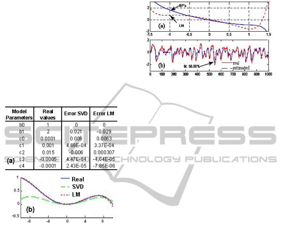
the model parameters estimated with our proposed
learning method LM after three training rounds
(which are sufficient for the algorithm to converge
provided the learning rate is appropriately selected).
These are compared with the SVD method (Lacy
2003). The results show that even though slightly
larger errors are obtained for b
1
and c
0
using the
proposed algorithm, all other parameter errors are
considerably better than those by the SVD method
(see Fig 2a). The model fit for the validation data
(not used in training) is 61.58% with the LM whilst
is only 38.22% with the SVD. The fitness to the real
output without noise is 96.41% for the LM and only
47.24% for SVD.
Figure 2: a) Errors in model estimates. b) Nonlinearity to
be identified.
Example 2. The LM algorithm was also applied to
the intracellular potential recorded from a spiking
local interneuron, that is part of the reflex control
loop of the hind limb (Newland et al 1997, Vidal-
Gadea et al 2009). The input signal was Gaussian
noise used to stimulate a stretch-sensor located at the
femoro-tibial joint of the hind leg. The noninvertible
nonlinearity identified using the proposed learning
method is shown in Figure 3a. The fitness for
validation data is 50.0% after three rounds of
training. The LM algorithm was also run in a BP-
like condition whereby the consideration of the
effect from the changing input (Remarks 1-3) was
removed. In this case, the fitness in the same
validation data is only 38.67% (three rounds of
training).. Here the model orders were N
a
=10, N
b
=30
and N
c
=9. Due to the high orders of the model, it is
difficult to apply the SVD method.
Figure 3: A practical example from a locust neuro
muscular control systems. (a) The estimated nonlinearity,
(c) Estimated ouput (LM).
5 CONCLUSIONS
Most of the existing algorithms for the identification
of Wiener models were developed under some
restrictive assumptions, such as white noise input,
part or full invertibility of the nonlinearity, or known
nonlinearity. A novel recursive algorithm based on a
learning approach has been developed for the
identification of Wiener systems with unknown and
noninvertible nonlinearity and noisy data. The new
algorithm can guarantee global convergence of the
estimation error to a small range around zero and is
easy to implement in a manner similar to the well-
known back propagation (BP) algorithm.
Comparisons between the proposed methodology
and existing algorithms such as SVD-based method
and BP algorithm were provided in two example
studies. The theoretical analysis and example studies
show the effectiveness and advantages of the
proposed approach. In continuing this work, we will
investigate optimal choices of the control parameters
for the algorithm, and provide more extensive
evaluations in simulated and recorded signals.
ACKNOWLEDGEMENTS
To BBSRC (UK) for financial support.
REFERENCES
Bai E., Reyland J., 2009. Automatica, 45:956-964
Billings S, Fakhouri S., 1978. Proceedings IEE 125:
961-697
Bloemen H., Chou C., van den Boom T, Verdult V.,
Verhaegen M., Backx T., 2001. Journal of Process
A LEARNING APPROACH TO IDENTIFICATION OF NONLINEAR PHYSIOLOGICAL SYSTEMS USING WIENER
MODELS
475

Control, 11: 601-620
Boyd S., Chua L., 1985. IEEE Trans. Circuits and
Systems, 32(11): 1150-1161
Figueroa J., Biagiola S., Agamennoni O.E, 2008.
Mathematical and Computer Modelling, 48:305–315
Gomez, J., Baeyens E, 2004. J. of Process Control, 14:
685-697
Greblicki W., 1997. IEEE Trans. Circuits and Systems. –
I: Fundamental Theory and Applications. 44, 538-545.
Kalafatis A.D., Wang L., Cluett W.R., 1997. International
Journal of Control, 66(6): 923-941
Kosmatopoulos E. and Polycarpou M., 1995. IEEE
Transactions Neural Networks. 6(2), 422-430.
Huang A. Tanskanen J.M.A., Hartimo I.O., 1998. Proc.
International Symposium Circuits and Systems,
5:249-252.
Hunter I., Korenberg M, 1986. Biol Cybernetics, 55: 135-
144
Jeffreys, H., Jeffreys, B., 1988. Methods of Mathematical
Physics, 3rd ed. Cambridge, England: Press, pp. 446-
448, 14.
Lacy S., Bernstein D., 2003. International Journal of
Control, 76(15), 1500-1507.
Narendra K.S., Gallman P.G, 1966., IEEE Tran Automatic
Control, 11(3): 546-550.
Nelies O., 2001. NewYork. Springer 1st Edition
Newland P., Kondoh Y., 1997. J.Neurophysiology 77:
1731-1746
Vidal-Gadea A., Jing X., Simpson D., Dewhirst O. Allen,
R. and Newland P, 2009. J. of Neurophysiology
103:603-615.
Wigren,T., 1993., Automatica 29 (4) 1011–1025
Wigren T., 1994., IEEE T Automatic Control, 38
(11):2191–2206
BIOSIGNALS 2011 - International Conference on Bio-inspired Systems and Signal Processing
476