
OPTICAL METHODS FOR LOCAL PULSE WAVE
VELOCITY ASSESSMENT
T. Pereira, M. Cabeleira, P. Matos, E. Borges, V. Almeida, J. Cardoso, C. Correia
Instrumentation Center, Physics Department, University of Coimbra, R Larga, Coimbra, Portugal
H. C. Pereira
Instrumentation Center, Physics Department, University of Coimbra, Coimbra, Portugal
ISA- Intelligent Sensing Anywhere, Coimbra, Portugal
Keywords: Optical probes, Photodiode, Waveform distension, Pulse Transit Time, Pulse Wave Velocity.
Abstract: Pulse wave velocity (PWV) is a clinically interesting parameter associated to cardiac risk due to arterial
stiffness, generally evaluated by the time that the pressure wave spends to travel between two arbitrary
points. Optic sensors are an attractive instrumental solution in this kind of time assessment applications due
to their truly non-contact operation capability, which ensures an interference free measurement. On the
other hand, they can pose different challenges to the designer, mostly related to the features of the signals
they produce and to the associated signal processing burden required to extract error free, reliable
information. In this work we evaluate two prototype optical probes dedicated to pulse transit time (PTT)
evaluation as well as three algorithms for its assessment. Although the tests were carried out at the test
bench, where “well behaved” signals can be obtained, the transition to a probe for use in humans is also
considered. Results demonstrated the possibility of measuring pulse transit times as short as 1 ms with less
than 1% error.
1 INTRODUCTION
Pulse wave velocity (PWV) is defined as the
velocity at which the pressure waves, generated by
the systolic contraction of the heart, propagate along
the arterial tree. PWV is a measure of regional
arterial stiffness of the arterial territory between the
two measurement sites. This parameter is related to
the elastic modulus (E) of the arterial wall (which
represents the intrinsic wall stiffness), and the
arterial geometry (thickness: h) and blood density
(ρ). The first relationship was formulated by Moens
and Korteweg and expresses:
ρ
d
Eh
PWV =
(1)
Later on, Bramwell and Hill described (1) the
association in terms of distensibility (D), which is
determined by the blood vessel’s compliance (C),
the former relation can be expressed:
DC
PWV
ρ
1
=
(2)
From the expression, we can deduce that higher
PWV corresponds to lower vessel distensibility and
compliance and therefore to higher arterial stiffness.
The pulse waves travel through the arteries at a
speed of 4 to 10 meters per second depending on the
vessel (PWV increases with the distance from the
heart), and the elastic condition of the arterial wall,
which is affected by a variety of factors in health
and disease (Bramwell, 1922; Nichols, 2005).
The most common technique to assess non-
invasively PWV is based on the acquisition of pulse
waves generated by the systolic ejection at two
distinct locations, separated by a distance d, and
determination the time delay, or pulse transit time,
due to the pulse wave propagation along the arterial
tree (Rajzer, 2008). The PWV parameter is then
simply calculated as the linear ratio between d and
the PTT.
74
Pereira T., Cabeleira M., Matos P., Borges E., Almeida V., Cardoso J., Correia C. and C. Pereira H..
OPTICAL METHODS FOR LOCAL PULSE WAVE VELOCITY ASSESSMENT.
DOI: 10.5220/0003166800740081
In Proceedings of the International Conference on Bio-inspired Systems and Signal Processing (BIOSIGNALS-2011), pages 74-81
ISBN: 978-989-8425-35-5
Copyright
c
2011 SCITEPRESS (Science and Technology Publications, Lda.)

Many different pulse waves have been used to
assess pulse wave velocity, such as pressure wave,
distension wave or flow wave. The gold standard in
PWV assessment uses pressure waves measured by
pressure sensors (Laurent, 2006). These sensors
need to exert pressure in the blood vessel this will
distort the waveform, and may lead to inaccurate
measurements. Another drawback of this method is
the fact that the predicted PWV is relative to a large
extension of the arterial tree and therefore is the
conjunction of different local PWVs.
Other studies describe ultrasonic probes that
predict PWV using Doppler Effect and modified
ecography probes (Minnan Xu, 2002), but the PWV
measurements were unreliable.
Recently (Kips et al, 2010; Vermeersch et al,
2008), described alternative approaches for
estimating carotid artery pressures with an
ultrasound system. Calibrated diameter distension
waveforms were compared to the more common
approach based on pressure waves, proving to be a
valid alternative to local pressure assessment at the
carotid artery.
All the previous techniques are minimally
invasive, but the probe has to be in contact with the
patient’s tissues at the artery site. This contact, as
stated above, can distort the signal integrity and thus
rise the interest in exploring true non-contact
technique.
The propagation of pressure waves in arterial
vessels generates distensions in the vessel’s walls.
These distensions can be optically measured in
peripheral arteries like the carotid that, as they run
very close to the surface impart a visible distention.
This distention, as it modulates the reflection
characteristics of the skin, can be used to generating
an optical signal correlated with the passing pressure
wave.
The probes developed in this work, gather the
light generated by LED illumination and reflected by
the skin, using two photodiodes placed 3 cm apart,
all assemble in a single probe. PWV is assessed by
measuring the time delay between the signals of the
two photo-sensors using different algorithms that are
also discussed.
2 TECNOLOGIES
Two distinct types of silicon optical sensors – planar
and avalanche photodiode (APD) – are used in this
work, each one requiring a particular electronic
circuitry. Results, however, are derived by the same
signal processing algorithms.
Each probe incorporates two identical optical
sensors placed 3 cm apart and signal conditioning
electronics based on a transconductance amplifier
and low-pass filter. The APD probe includes the
high voltage biasing circuitry (250V) necessary to
guarantee the avalanche effect. Illumination is
provided by local, high brightness, 635 nm light-
emitting diodes (LEDs).
A photodiode (PD) is a type of photo-detector
with the ability of converting light into either current
or voltage, according to the modus operandi. One
decided to use a planar, rectangular-shaped
photodiode, its dimensions being 10.2x5.1mm. This
is silicon solderable photodiode feature low cost,
high reliability and a linear short circuit current over
a wide range of illumination.
Analogously to the conventional photodiodes,
APDs operate from the electron-hole pairs created
by the absorption of incident photons. The high
reverse bias voltage of APDs, however, originates a
strong internal electric field, which accelerates the
electrons through the silicon crystal lattice and
produces secondary electrons by impact ionization.
This avalanche effect is responsible for a gain factor
up to several hundred.
APDs are operated with a relatively high reverse
voltage and will typically require 200 to 300 volts of
reverse bias. Under these conditions, gains of around
50 will result from the avalanche effect, providing a
larger signal from small variations of light reflected
from the skin and will, at least theoretically, improve
the signal-to-noise ratio (SNR).
On the other hand, since the sensitive area of this
sensor is very small (1 mm
2
), the accuracy of the
estimations increases. In fact, comparatively to the
planar photodiode, in which the detection of light
takes place over a much larger area, this sensor can
measure an almost punctual section of the skin, thus
decreasing the error associated to the detection solid
angle.
The two prototype probes, on which we support
this work, incorporate an APD from Adavanced
Photonics (SD 012-70-62-541) and a planar type
from Silonex (SLCD-61N3) respectively.
3 TEST SETUP
The test setup was designed to assess the two main
parameters of in PWV measurements: linearity and
time resolution.
Their assessment was carried out in a test setup
where illumination is provided by two LEDs whose
light intensities reproduce the same signal with a
OPTICAL METHODS FOR LOCAL PULSE WAVE VELOCITY ASSESSMENT
75
variable time delay between them, as shown in
Figure 1.
Two arbitrary waveform generators, Agilent
33220A (AWG1 and AWG2), are synchronously
triggered by an external signal. The waveform
generators have been previously loaded with the
same typical cardiac waveforms and the mutual
delay is selected in order to simulate different pulse
transit times (Figure 2). These signals must be added
to a small offset of the order of the magnitude of the
forward voltage drop of the LED, so that the
resulting light intensity is linearly modulated by the
LED signal current. A 16-bit resolution data
acquisition system (National Instruments, USB6210)
samples the signals at a 20 kHz rate, adequate for
PTTs as low as 100 µs and stores them for off-line
analysis using MatlabTM.
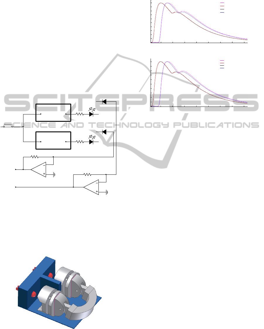
Figure 1: Light modulation and detection circuit.
In the test setup, the probe is placed in front of a
test device, see Figure 2, which holds the two
modulated LEDs and provides light isolation to
prevent crosstalk. During the tests, the LEDs of the
probe itself are deactivated and all light comes from
the LEDs in the test device.
Figure 2: During test, the probe is held to the blue part.
The test LEDs activated by circuit of Figure 1.
Figure 3 shows a typical set of signals generated and
detected by the circuit of Figure 1.
a)
b)
Figure 3: Excitation and detector responses for a) Planar
Photodiode b) Avalanche Photodiode.
To assess the operational limits of our probes and
algorithms, we designed three different tests. In the
first one, signals with frequency similar to the
normal heart rate but with delays within the
interesting PTT range are fed to the system to
investigate the integral linearity error. This test was
performed at a constant frequency of 1.5 Hz and
time delays varying from 1ms to 100ms,
corresponding to PWVs in a 30m/s to 0.3m/s
interval. This range of values includes the normal
PTT range of values in humans.
In the second test we assess the robustness of the
algorithms to noise. To do this, we add white noise
of amplitudes ranging from 1% to 50% of the signal
amplitude in 0.02% steps, to the isolated pair of
pulses. For each noise level, 1000 samples produced
in order to obtain reasonable statistics. The resulting
PTT distribution is then studied.
The third test was intended to validate our
algorithm’s operability under a wide range of
frequencies (simulating different Heart rates) with a
time lag far greater than the maximum PTT seen in
humans. It consisted of varying the output frequency
(1 Hz to 200 Hz) of the cardiac pulses keeping the
time lag between the two signals at 1.1ms.
Trigger
L1
L2
PD1
PD2
U1
U2
AWG1
AWG2
0.05 0.1 0.15 0.2 0.25 0. 3 0. 35 0.4
0
0.1
0.2
0.3
0.4
0.5
0.6
0.7
0.8
0.9
1
Time [sec]
Amplitude [A.U.]
Signal Sensor 1
Signal Sensor2
Signal LED 1
Signal LED 2
0.05 0.1 0.15 0.2 0.25 0.3 0.35 0.4
0
0.1
0.2
0.3
0.4
0.5
0.6
0.7
0.8
0.9
1
Time [sec]
Amplitude [A.U.]
Signal Sensor 1
Signal Sensor2
Signal LED 1
Signal LED 2
R
T
R
T
R
M
R
M
BIOSIGNALS 2011 - International Conference on Bio-inspired Systems and Signal Processing
76

4 SIGNAL PROCESSING
Three different algorithms for extracting the time
delay from the detector’s signals are considered.
They are referred to as foot-to-foot, cross-correlation
and phase spectra. Their basis derives from the
homonymous mathematical functions.
The accuracy of the results delivered by the
algorithms discussed in this section is compared
with the reference delay selected at the waveform
generators.
In the foot-to-foot method and in spite of more
complex methods (Kazanavicius, 2005), a simple
detection of the time lag between the start of the
upstroke of the two consecutive pulses is carried out.
This is possible due to the well behaved nature and
low noise levels of our signals. A different situation
occurs in signals collected from a patient, mostly
due to baseline drift.
The cross-correlation method is based on the
well known property of the peak of cross-
correlogram that allows delays to be calculated by
subtracting the peak time position from the pulse
length (Azaria, 1984). Two different correlation
functions are used: one that belongs to the
MatlabTM core (Xcorr) and another one that
generates the cross-correlation making direct use of
the cross-correlation theorem (Fcorr).
The third method uses data in the phase spectra
of the signals. In this method, we first identify the
exact frequency of the signal’s harmonics, using the
amplitude spectra, and then, extract the
corresponding phase angles from the phase spectra.
The phase angle, θ, is related with angular
frequency of the phase spectrum, ω and with the
time delay, t, according to:
t⋅=
ω
θ
(3)
On its turn, the time delay is computed from the
phase angles of the same harmonic in the phase
spectra of each signal, θ
1
and θ
2
:
(
)
ω
θ
θ
21
−
=t
(4)
Despite the fact that, theoretically, the time delay
can be determined at any harmonic of the complete
spectrum, the practice, however, differs, given their
affectation by noise. Nevertheless, by performing
the filtering at the detector amplifier level, one is
able to obtain a lower error, as long as the best
harmonics (that is, with the highest SNR possible)
are selected. For the circuits used in this study, one
checked best performances when the time delay was
computed at the 2nd harmonic in the APD case and
in the 4th one for the PP circuits.
5 RESULTS
This section is dedicated to the discussion of results
obtained with the two probes using the previously
mentioned algorithms.
5.1 Integral Linearity
By definition, integral linearity is the maximum
deviation of the results from the reference straight
line, expressed as a percentage of the maximum. We
explore delays in the 1 to 100 ms interval. Results
are shown in Figures 4 and 5.
A higher number of points are taken close to the
origin since this is the interesting range of values in
human PTT studies using the optical probes.
Figure 4: Reference Delay versus measured delay for the
PP probe. The APD curve practically coincides with this
one.
For both probes, all the algorithms produce highly
linear (better than 1%) results as well as low error
agreement with the reference time delay.
5.2 PTT Error
Error plots, expressed as a percentage of the
corresponding reference value, are shown in Figures
5 and 6. We discuss the main differences between
the PP and the APD probes.
y = 1,0067x -0,0002
R² = 1
0
0,01
0,02
0,03
0,04
0,05
0,06
0,07
0,08
0,09
0,1
0 0,02 0,04 0,06 0,08 0,1
Time Delay [sec]
Reference Time Delay [sec]
Xcorr Fcorr Foot Phase
OPTICAL METHODS FOR LOCAL PULSE WAVE VELOCITY ASSESSMENT
77
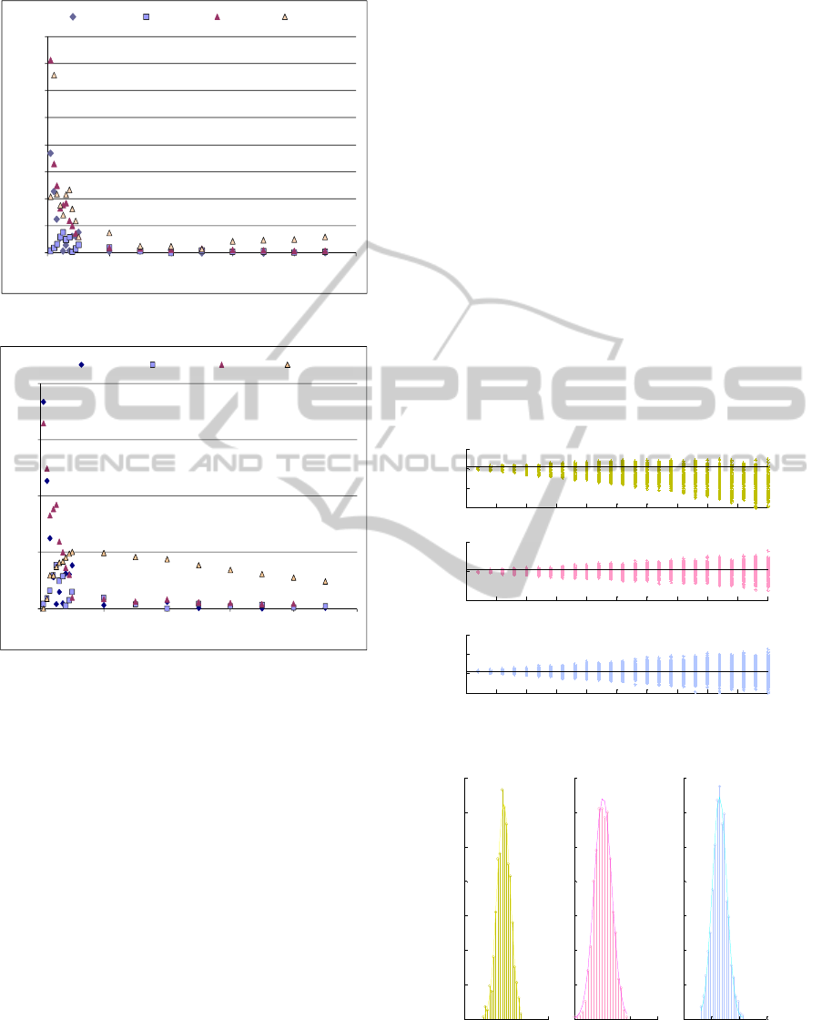
Figure 5: Relative errors by algorithm, for the PP probe.
Figure 6: Relative errors, by algorithm, for the APD probe.
While the PP probe exhibits lower than 8% error,
the APD one never exceeds the 4% limit.
Cross-correlation (Fcorr version) can be
identified as the best performing algorithm with a
relative error never exceeding 1% in any probe.
In the APD probe, the phase angle detection
method also yields very good (lower than 1%) error,
but poor performance for the PP probe, mainly in the
small time lag region.
As expected all the algorithms performed almost
perfectly for higher than 10ms time delays.
5.3 Noise Tolerance
Robustness of the algorithms to noise is assessed by
adding normal distribution noise to the photodiode
readings and studying the resulting effect on the
algorithm output.
This test was performed just for the correlation
and phase methods. It was not used in foot-to-foot
detection, because, as long as added noise is of the
order of magnitude of the threshold used to detect
the upstroke, the upstroke will not be detected at all.
Data collected by the PP and APD probes was
submitted to this test using the following procedure:
for each noise level, the algorithm under test was run
1000 times, with an independent noise vector
affecting every run.
In total, 25 relative noise levels, from zero to 0.5
of peak amplitude, were explored.
Figures 7 to 12, enclosing the full information of
this test, are shown side by side to make
comparisons easier.
Figures 8 and 9 show the dispersion introduced
by noise for a reference delay of 4.1 ms. The
resulting PTT values, taken as the mean value of
each distribution, are plotted in Figure 9. While
these figures concern the PP probe, Figures 10, 11
and 12 represent the same study for the APD probe.
As mentioned before, noise is expressed as a
fraction of the peak amplitude of the signal.
Figure 7: Dispersion introduced by noise in the PP probe.
Figure 8: PTT dispersion plots for each algorithm, for a
relative noise level of 0.14. The gaussian fittings stress the
normal nature of the distributions.
0%
1%
2%
3%
4%
5%
6%
7%
8%
0 0,02 0,04 0,06 0,08 0,1
Erro r [%]
Reference Time Delay [sec]
Xcorr Fcorr Foot Phase
0%
1%
2%
3%
4%
0 0,02 0,04 0,06 0,08 0,1
Error [%]
Reference Time Delay [sec]
Xcorr Fcorr Foot Phase
0 0.05 0.1 0.15 0.2 0.25 0.3 0.35 0.4 0.45 0.5
2
3
4
5
x 10
-3
Xcorr
0 0.05 0.1 0.15 0.2 0.25 0.3 0.35 0.4 0.45 0.5
2
4
6
x 10
-3
Fcorr
Time [sec]
0 0.05 0.1 0.15 0.2 0.25 0.3 0.35 0.4 0.45 0.5
3
4
5
6
x 10
-3
Phase
Relative noise
3.5 4 4.5 5
x 10
-3
0
20
40
60
80
100
120
140
Time [sec]
Phase
3.5 4 4.5 5
x 10
-3
0
20
40
60
80
100
120
140
Time [sec]
Fcorr
3 4 5
x 10
-3
0
20
40
60
80
100
120
140
Time [sec]
Xcorr
BIOSIGNALS 2011 - International Conference on Bio-inspired Systems and Signal Processing
78
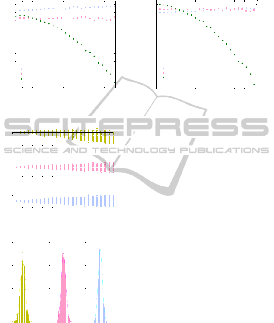
Figure 9: Mean of distribution vs. relative noise for a 4.1
ms reference delay in the PP probe.
Figure 10: Dispersion introduced by noise for the APD
probe.
Figure 11: PTT dispersion plots for each algorithm, for a
relative noise level of 0.14. The gaussian fitting stresses
the normal nature of the distribution.
Figure 12: Mean of distribution vs. relative noise for a 4.1
ms reference delay in the APD probe.
Not surprisingly, the dispersion introduced by
adding noise is also gaussian with variance
proportional to the noise level (Figures 8 and 11).
However, different robustness to noise is
exhibited by each of the three tested algorithms, with
the phase and Fcorr methods showing the lowest
errors when subject to high levels of noise.
It is also clear that the Xcorr based algorithm is
not robust to noise and, under high noise conditions
it shows a strong tendency to under-evaluate PTT, as
shown in Figures 9 and 12.
The phase method exhibits the higher levels of
robustness since its median remains constant for
high noise levels and, in addition, the corresponding
distribution shows the lower variance. The large
offset yielded by this algorithm in the PP probe (but
not in the APD probe) is rather puzzling and is
probably associated to the particular shape of PP
signals which, very much unlike the APD, are
conditioned by the large equivalent capacity of the
photosensor.
Another clarifying way to look at the overall
performance of probes and algorithms is shown in
Figure 13 where the probabilities of the algorithm
returning a PTT value with less than 5% and less
than 10% error are plotted against noise. Results,
expressed as a percentage, are derived from 1000
runs per curve.
Data in Figure 13 confirms the superior
robustness of the phase method.
0.05 0.1 0.15 0.2 0.25 0.3 0.35 0.4 0.45 0.5
3.2
3.3
3.4
3.5
3.6
3.7
3.8
3.9
4
4.1
4.2
x 10
-3
Relative noise
Time [sec]
Phase
Fcorr
Xcorr
0 0.05 0.1 0.15 0.2 0.25 0.3 0.35 0.4 0.45 0.5
2
3
4
5
x 10
-3
Xcorr
0 0.05 0.1 0.15 0.2 0.25 0.3 0.35 0.4 0.45 0.5
2
4
6
x 10
-3
Fcorr
Time [sec]
0 0.05 0.1 0.15 0.2 0.25 0.3 0.35 0.4 0.45 0.5
3
4
5
6
x 10
-3
Phase
Relative noise
2 4 6
x 10
-3
0
20
40
60
80
100
120
140
Time [sec]
Phase
2 4 6
x 10
-3
0
10
20
30
40
50
60
70
Time [sec]
Fcorr
2 4 6
x 10
-3
0
10
20
30
40
50
60
70
Time [sec]
Xcorr
0.05 0.1 0.15 0.2 0.25 0.3 0.35 0.4 0. 45 0.5
3.4
3.5
3.6
3.7
3.8
3.9
4
4.1
4.2
x 10
-3
Relative noise
Time [sec]
Phase
Fcorr
Xcorr
OPTICAL METHODS FOR LOCAL PULSE WAVE VELOCITY ASSESSMENT
79
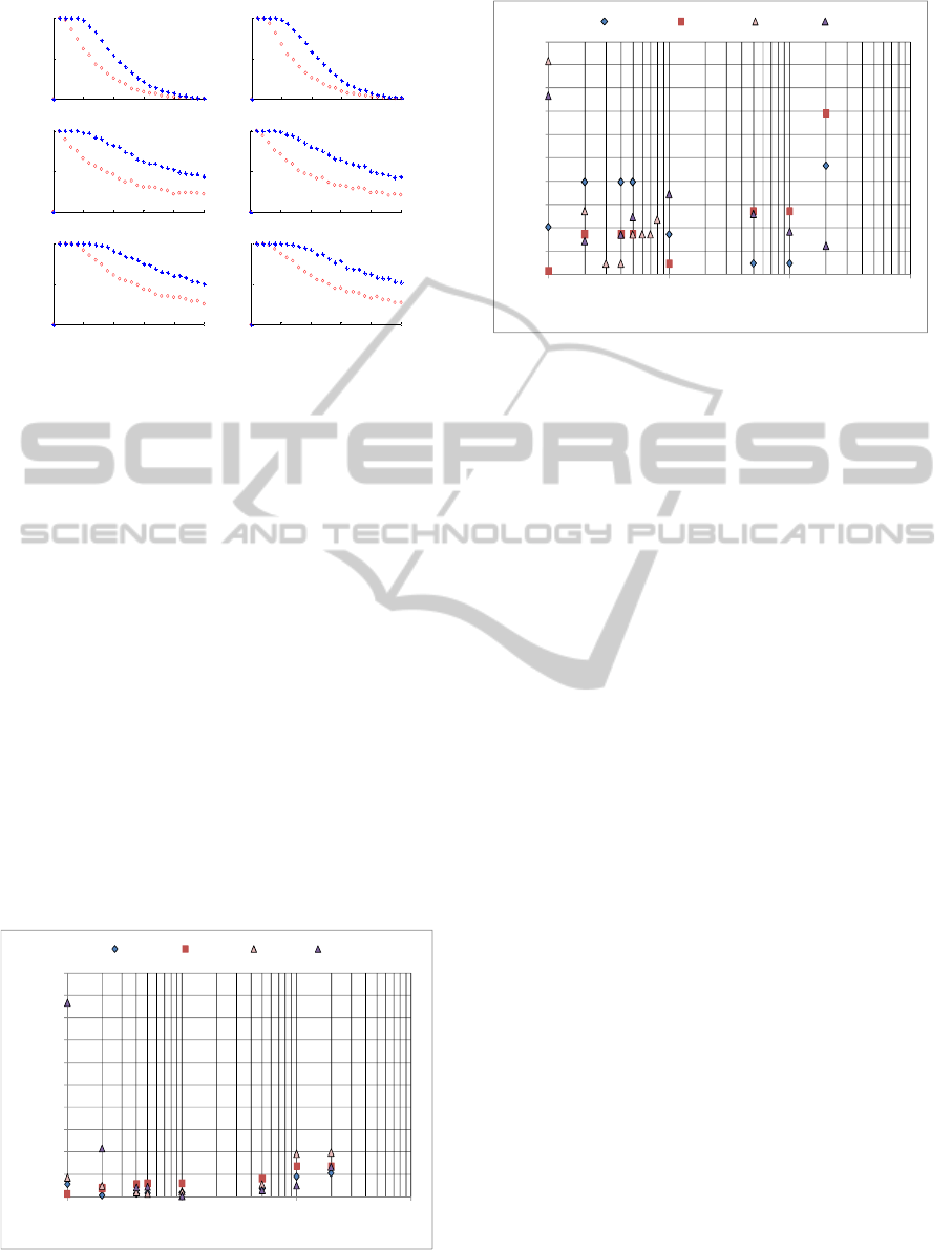
Figure 13: Measurements with less than 5% error (blue
dots) and less than 10% error (red circles) vs. relative
noise.
As can be stated, all algorithms can deliver 100%
measurements within the specified error threshold,
up to a certain noise level, where the curves show a
turning point and start decaying towards zero. The
phase algorithm not only shows a higher turning
point but also decays much slowly as noise
increases, denoting extra robustness to noise.
5.4 Algorithm Robustness
A final test was carried out in order to study the
effect of different heart rates on the performance of
the algorithms. In fact, all the data mentioned so far
was acquired at a rate of 1 pulse per second, thus,
any conclusive notes might not be valid for other
acquisition rates. Accordingly, the referred test was
performed for signal repetition rates varying from 1
to 200 Hz, without artificial noise added to the
readings and for a known constant time delay.
Figure 14: Plot of the relative errors for each algorithm for
a range of frequencies of signal, for the PP probe.
Figure 15: Plot of the relative errors for each algorithm for
a range of frequencies of signal, for the APD probe.
The value used for the time delay, 1.1 ms, was
selected by mere convenience. At this point it’s not
unimportant to remark that the AWG2 (Figure 1)
can define the time delay as an angle, the delay
angle, with a precision of a tenth of a degree; on the
other side, for the specific used set of repetition
rates, the value of 1.1 ms yields feasible values for
delay angles that, otherwise, could not be loaded by
the equipment.
In conclusion, as Figures 14 and 15 reveal, the
APD probe performs superiorly (note that the
vertical scales of the figures are different). It is also
noticeable that the Fcorr and the phase algorithms
produce the best results if the entire range of
repetition rates is considered.
6 CONCLUSIONS
Two optical probes specifically designed to measure
PTT have been developed and tested along with
three different signal processing algorithms.
Tests show that although both probes are capable
of measuring PTT accurately, the APD based one is
more precise and accurate.
All three tested algorithms can measure PTT
with an error below 8%. Nevertheless, just the one
designated by Fcorr exhibits the capability of
measuring PTT with an error bellow 1%, for the
complete range of delays. The phase method shows
the higher levels of robustness to noise.
When the signal repetition rate spans over a large
range of values, the Fcorr algorithm can deliver
PTTs with the lowest errors.
The natural follow-up of this work will be start
acquiring pulse data in humans. Figure 16 shows a
preliminary acquisition in human using the APD
0 0.1 0.2 0.3 0.4 0.5
0
50
100
PPD - Xcorr
0 0.1 0.2 0.3 0.4 0.5
0
50
100
PPD - Fcorr
Time [sec]
0 0.1 0.2 0.3 0.4 0.5
0
50
100
PPD - Phase
Relative noise
0 0.1 0.2 0.3 0.4 0.5
0
50
100
APD - Xcorr
0 0.1 0.2 0.3 0.4 0.5
0
50
100
APD - Fcorr
0 0.1 0.2 0.3 0.4 0.5
0
50
100
APD - Phase
Relative noise
0%
10%
20%
30%
40%
50%
60%
70%
80%
90%
100%
1 10 100 1000
Error [%]
Repetition rate [Hz]
Xcorr Fcorr Foot Phase
0%
2%
4%
6%
8%
10%
12%
14%
16%
18%
20%
1 10 100 1000
Error [%]
Repetition rate [Hz]
Xcorr Fcorr Foot Phase
BIOSIGNALS 2011 - International Conference on Bio-inspired Systems and Signal Processing
80
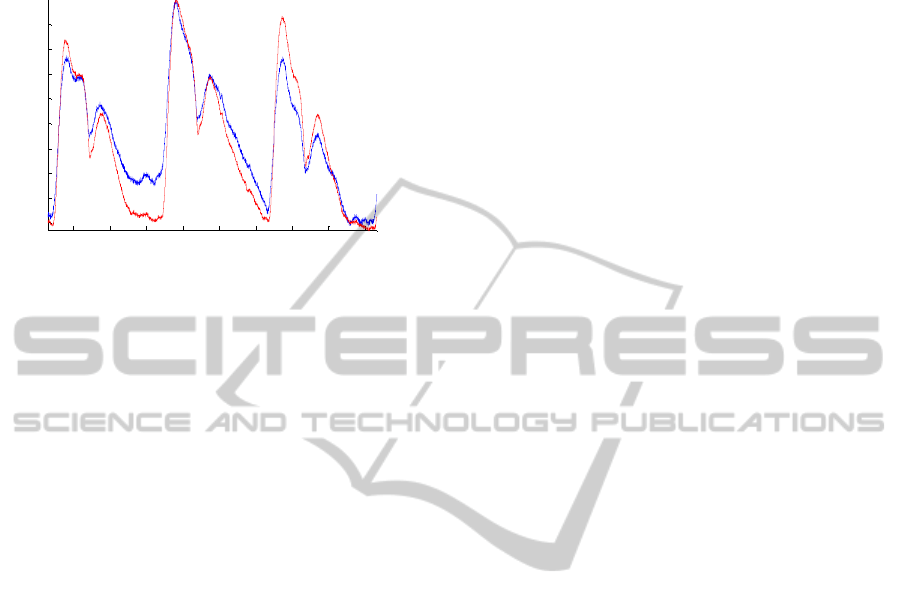
probe. The shape of the pulses is very clear, not to
much affected by noise and allows the anticipation
of good results.
Figure 16: Preliminary results of the APD probe acquiring
data in humans.
ACKNOWLEDGEMENTS
The authors acknowledge the support from
Fundação para a Ciência e Tecnologia (FCT) for
funding (PTDC/SAU-BEB/100650/2008).
REFERENCES
Laurent S, et al., 2006. Expert consensus document on
arterial stiffness: methodological issues and clinical
applications Eur Heart. J. 27 2588-2605.
Kips J, et al., 2010. The use of diameter distension
waveforms as an alternative for tonometric pressure to
assess carotid blood pressure. Physiol. Meas. 31
(2010) 543–553.
Vermeersch S. J. et al., 2008. Determining carotid artery
pressure from scaled diameter waveforms: comparison
and validation of calibration techniques in 2026
subjects. Physiol. Meas. 29 1267–80.
Minnan Xu, 2002 Local Measurement of the Pulse Wave
Velocity using Doppler Ultrasound. Massachusetts
Institute of Tecnology.
Bramwell J. and Hill A., 1922. The velocity of the pulse
wave in man. Proc Roy Soc Lond [Biol]. 93 298-306
Nichols, W. and O’Rourke, M. F., 2005. McDonald’s
Blood Flow in Arteries: Theoretical Experimental and
Clinical Principles. 5th ed., London.
Rajzer M. et al., 2008. Comparison of aortic pulse wave
velocity measured by three techniques: Complior,
Spymocor and Arteriograph. J. Hypertens. 26
2001:2007.
Azaria M. and Hertz D., 1984. Time delay estimation by
generalized cross correlation methods. IEEE Trans.
Acoustics, Speech, and Signal Processing, vol. ASSP-
32, pp. 280-285.
Kazanavicius E. and Gircys R., 2005. Mathematical
Methods for determining the foot point of the Arterial
Pulse Wave and Evaluation of Proposed Methods.
ISSN 1392 – 124X Information Technology and
Control.
0.5 1 1.5 2 2.5 3 3.5 4 4.5
x 10
4
0.1
0.2
0.3
0.4
0.5
0.6
0.7
0.8
0.9
Time [sec]
A.U.
OPTICAL METHODS FOR LOCAL PULSE WAVE VELOCITY ASSESSMENT
81
