THE DYNAMICS OF LOCUST NON-SPIKING LOCAL

INTERNEURONS

Responses to Imposed Limb Movements

Oliver P. Dewhirst, Natalia Angarita-Jaimes, David M. Simpson, Robert Allen

Institute of Sound and Vibration Research, University of Southampton, Southampton, SO17 1BJ, U.K.

Philip L. Newland

School of Biological Sciences, Building 85, University of Southampton, Highfield Campus, Southampton, SO17 1BJ, U.K.

Keywords: Reflex Dynamics, Nonlinear System Identification, Wiener Laguerre.

Abstract: A key feature of the locusts hind leg control system is a reflex loop that uses a stretch sensor, the Femoral

Chordotonal organ, to monitor the position and movements of the tibia relative to the femur. A population

of non-spiking local interneurons in the metathoracic ganglia receive synaptic inputs from the sensory

neurons in the chordotonal organ and indirect inputs from other interneurons. They function to integrate

these signals and generate the motor pattern required for coordinated limb movement. Nonlinear Volterra

models combined with Gaussian white noise stimulation have, for the first time, been used to characterise

the dynamics of this population of interneurons. The results show that the interneurons can be clustered into

three groups, those which are position, position/velocity and velocity sensitive.

1 INTRODUCTION

Reflexes are a critical part of vertebrate and

arthropod motor control systems allowing posture

and movement to be adapted to changes in the

external environment. Greater understanding of the

reflex control of limb movement should allow the

features of such systems to be exploited to improve

the design of engineering control systems (bio-

inspired design) (Bar-Cohen, 2006). Arthropods

provide an opportunity to develop new investigative

techniques and gain insight into a relatively simple

and accessible neuromuscular reflex control system.

Three ganglia in the locusts thorax contain neurons

responsible for controlling movements of the legs

(Figure1). A key feature of its hind limb reflex

control system is a stretch sensor called the Femoro-

tibial Chordotonal Organ (FeCO) (Burrows, 1996).

This sensor monitors the movement of the tibia

about the femoro-tibial joint (Figure 1). Movements

of the tibia are converted into action potentials by

sensory neurons located in the FeCO (~90 cells).

These signals are processed by spiking local

interneurons and then integrated with information

from other sensors by the non-spiking local

interneurons. The non-spiking local interneurons

transmit this information using graded potentials to

the leg motor neurons which activate muscle

contraction (Burrows, 1996). It is believed that the

non-spiking interneurons have the ability to

modulate the reflex response in one limb given

information integrated from both local sensors and

those on other limbs and hence play a crucial role in

the production of coordinated limb movement

(Burrows, 1996). Previous work has described the

connections between the non-spiking local

interneurons and the motor neurons in the hind leg

of the locust (Laurent and Burrows, 1989). Little is

known, however, of the range of inputs received by

these interneurons. In this paper a nonlinear Volterra

model combined with a Gaussian White Noise

(GWN) stimulation signal has been used to

characterise the input sensitivity of a population of

non-spiking local interneurons to imposed

movements of the locust hind leg femoro-tibial joint.

A similar technique has been used to model a

population of spiking local interneurons (Vidal-

Gadea et al., 2009).

That study, however, used the Wiener series and

a cross correlation parameter estimation method

270

Dewhirst O., Angarita-Jaimes N., M. Simpson D., Allen R. and L. Newland P..

THE DYNAMICS OF LOCUST NON-SPIKING LOCAL INTERNEURONS - Responses to Imposed Limb Movements.

DOI: 10.5220/0003168002700275

In Proceedings of the International Conference on Bio-inspired Systems and Signal Processing (BIOSIGNALS-2011), pages 270-275

ISBN: 978-989-8425-35-5

 2011 SCITEPRESS (Science and Technology Publications, Lda.)

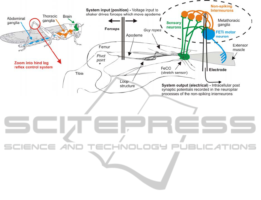
Figure 1: The locust hind leg control system and the non-spiking local interneurons modelled in this study.

(Schetzen, 1981). Whilst the cross correlation

method is relatively computationally efficient, its

accuracy relies on the properties of the input signal

(Westwick et al., 1998). Parameter estimation

accuracy is improved in the current study by

estimating the parameters of a Volterra model using

a Least Squares technique. Model complexity is

significantly reduced using Laguerre basis functions

(Marmarelis, 1993).

2 METHODS

2.1 Experimental Methods

Experiments were performed on 11 adult male and

female desert locusts, Schistocerca gregaria

(Forskål) at room temperature (21.5±°C, relative

humidity 35.7±3.7%). Locusts were mounted ventral

side uppermost in modelling clay. The apodeme of

the FeCO (Figure 1) was exposed and attached by

forceps to a shaker (Ling Altec 101). The FeCO was

stimulated by applying a 27Hz low pass filtered

GWN signal to the shaker (CG-742, NF Circuit

Design Block). Intracellular recordings were made

using a glass microelectrode which was inserted into

the neuropillar processes of the interneurons in the

metathoracic ganglia. The synaptic potentials were

amplified using an Axoclamp 2A amplifier (Axon

Instruments). Signals were stored on magnetic tape

(digital format) using a PCM-DAT recorder (RD-

101T, TEAC) operating at a sampling rate of

24KHz. The data were transferred to a computer

using a PCMCIA interface card and QuikVu

software (TEAC) and analysis was carried out using

MATLAB (Mathworks, Cambridge UK).

2.2 Signal Processing: Theory

The second order Volterra series is written as

011 1

212 1 2

() ( )( )

( , )( )( )

yn h h un

hunun

ττ

τττ

−

−−

=+ − +

−−

∑

∑∑

(1)

where

)(nu

is the input;

()h

and

),(

212

are the zero, first and second order

kernels and L is the number of lags. To facilitate

parameter estimation, Wiener (1958) expressed the

series in terms of a set of orthogonal functions:

011

212 12

() ( ) ()

(, )

nc c

cjj

ϑϑ

−

−−

∑

∑∑

(2)

where J is the number of functions in the

decomposition and c are the coefficients of the

Wiener kernels. The orthogonal basis functions

)(n

are obtained using

∑

−=

mnumLn

)()()(

(3)

()

() ( )

1/2

() 1

αα

−

=−

⎛⎞⎛⎞

−−

⎜⎟⎜⎟

⎝⎠⎝⎠

∑

(4)

where

is the

order Laguerre function and

is the “decay parameter” controlling the damping of

the Laguerre function. A lag of 100ms,

=0.5 and J

THE DYNAMICS OF LOCUST NON-SPIKING LOCAL INTERNEURONS - Responses to Imposed Limb Movements

271

= 6 were required to capture the dynamics of the

interneurons. The outputs of the series can be

calculated recursively using

() () ( )

11)(

−−+−=

−−

nnnn

jjjj

ϑϑαϑαϑ

(5)

with

)(

defined as:

()

)(11)(

nuTnn

αϑαϑ

−+−=

(6)

where T is the sampling interval. The

coefficients

)( jc

(Equation 2) were calculated from

the basis functions using the Least Squares method.

The kernels were then obtained using

11 1 1

212 212 1 22

() () ()

(, ) (, ) () ()

hcjL

hcjjLL

ττ

τττ

−

−−

=⋅

=⋅⋅

∑

∑∑

(7)

2.3 Signal Processing: Application

Our analysis is based on that used in similar studies

(Newland and Kondoh, 1997a and Vidal-Gadea et

al., 2009) on different neurons. Models were fitted

between the first 20 seconds of steady state adapted

response (Figure 2B s3) and the corresponding

samples of input signal. Validation was carried out

using the last 4s of the recording by calculating the

fitness function (Figure 2B s4).

()

100 1 ( ) ( ) / ( ))

it yt yt yt=×− −

(8)

where

•

is the Euclidean norm (mean square

value),

()yt is the measured output and

()yt

is the

predicted output. In order to study patterns in the

interneuron’s responses kernels were clustered using

the K-means algorithm (Hartigan and Wong, 1979).

In order to focus on their sensitivity to position,

velocity and acceleration (of primary interest to

neurophysiologists), the gradient m of a linear

function y=mx+c fitted to the frequency response

(magnitude only) calculated from the first order

kernel between 2 and 15Hz was used as the feature

for the k-means algorithm. The interpretation of the

linear kernels is illustrated in Figure 3A and B. A

position sensitive model has a kernel with a

monophasic impulse response and flat frequency

response. A velocity sensitive model has a biphasic

kernel and a frequency response with a linear

increase (20dB/decade, Figure 3B). A triphasic

impulse response indicates an acceleration sensitive

interneuron (40dB/decade, Figure 3B). Whilst the

first order kernel provides a means to describe the

linear dynamic sensitivity of the interneurons, the

majority of the interneurons have a nonlinear

response, such as being primarily excitatory or

inhibitory, or more sensitive to extension or flexion.

Figure 2: The band limited (0-27Hz) GWN input signal

(A). The typical response of an interneuron (B) with

spontaneous activity (s1), transient adapting (s2), steady

state adapted response (s3) and validation section (s4).

This is illustrated in Figure 3C where the response of

a model of an interneuron to sinusoidal movement of

the tibia is shown. It should be noted that the linear

model gives equal sensitivity to both flexion and

extension, with inhibition during flexion and

excitation during extension. The response of the

nonlinear model, however, shows how this

interneuron is only weakly inhibited during flexion

of the leg but has a strong excitatory input when the

leg is extended. The response to such a sinusoid will

be used to illustrate the overall (linear and nonlinear)

response of the neuron.

Figure 3: Illustrative 1

order kernels (A) and gain curves

(B) showing position (P), velocity (V) and acceleration

(Acc) sensitive models. Typical model response to a 6Hz

sinusoidal input signal is shown in (C).

BIOSIGNALS 2011 - International Conference on Bio-inspired Systems and Signal Processing

272

3 RESULTS

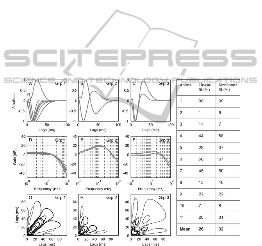
The linear dynamics of the 11 interneurons clustered

into three groups according to the sensitivity of their

responses to position, velocity or acceleration is

shown in Figure 4. Clearly the idealized patterns in

Figure 3B are not observed, but consistent patterns

that indicate a range of sensitivities are evident in

Figure 4D-F. The models of the interneurons in

group 1 (Figure 4A, D) show a monophasic 1

order

kernel. They have a flat frequency response in the

range 0-20Hz and a decrease of -30dB/dec > 20 Hz

indicating that interneurons in this group are

primarily position sensitive. The models in groups 2

and 3 show a biphasic first-order kernel and a

positive slope in their frequency response between

0-20Hz indicating that they mainly responded to the

rate of change of movement of the stimulus. The two

groups, however, differ in their response at lower

frequencies. Whilst the models in group 2 show a

constant slope in their frequency response (~20dB

/dec), in group 3 the responses are flatter at lower

frequencies (0-3Hz) followed by a positive slope

from ~3-20Hz (6dB/dec). No clearly acceleration

sensitive interneuron models were found in this

study. The second order kernels are shown in Figure

4G to I. The majority of interneurons in group 1

(Figure 4G) have a long positive excitatory peak

along the diagonal line of their 2

order kernel

(Figure 4G) and a dominant negative peak in their

first order kernel (Figure 4A).

Interneurons in the 2

and 3

groups have

second-order kernels with a main inhibitory area (or

excitatory depending on the direction of the

dominant peak of the linear response) that are

smaller compared to those in group 1 (Figure 4H, I).

Also, these dominant areas peak closer to the origin

reinforcing the hypothesis that these interneurons

respond faster to stimulus changes.

An initial positive peak of the first order kernel

Figure 4: The impulse responses of the 1

order Volterra kernels of 11 interneurons separated into three groups using the K

means clustering algorithm (A-C). Impulse responses have been normalised to unit peak value. The monophasic impulse

response (A) and flat frequency response (D) indicate that group 1 is position sensitive. The biphasic impulse response (B

and C) and positive slopes in the frequency response indicate that groups 2 and 3 are more velocity sensitive. The 2

order

Volterra kernels (G-I), positive values are represented by a thick line, negative values by a thin line. The kernels from group

1 are shown in G and have a dominant elongated peak along the diagonal. The kernels from groups 2 and 3 are shown in H

and I respectively. They have dominant deflections closer to the origin than those in group 1 and are therefore faster to

respond to stimulus changes. The predictive accuracy (fit) of the linear and nonlinear models is shown in the table.

THE DYNAMICS OF LOCUST NON-SPIKING LOCAL INTERNEURONS - Responses to Imposed Limb Movements

273

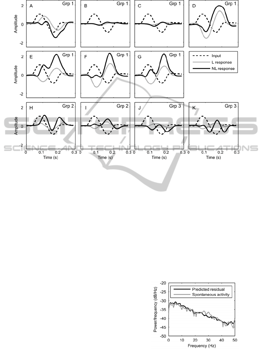
Figure 5: The response of the linear (L, first order kernel) of the nonlinear model and the nonlinear response of the model

(NL, combined response of the first and second order kernels) to one period of a 6Hz sinusoidal input signal.

indicates that a neuron is excited during flexion and

inhibited during extension. An initial negative phase

would indicate excitation during extension and

inhibition during flexion. In order to get the

complete picture of the neurons characteristic,

however, the response of the nonlinear model must

be added. The effect that the first (linear) and the

combined first and second order (nonlinear) kernels

from group 1 have on a 6Hz sinusoidal input is

shown in Figure 5A-G. The linear component gives

equal sensitivity to both flexion and extension with

inhibition during flexion and excitation during

extension in 6 out of 7 cases (Figure 5A is the

exception). When combined (linear + nonlinear)

responses are taken, however, the interneurons in

Figure 5E, F and G no longer respond with strong

inhibition during flexion, and those in Figure 5D, E,

F and G are strongly excitatory during extension.

There would appear to be less consistency in the

responses of the non-spiking local interneurons in

groups 2 and 3.

The performance of the Volterra models was

evaluated by comparing the predicted response

given by the models and the response (synaptic

potential) recorded from the non-spiking local

interneurons. Model fit was calculated using

validation data. The fit of the linear (first order) and

the nonlinear (first + second order) models for the 11

interneurons is shown in Figure 4. In some cases

(especially for animals 2, 3 and 10) the fit is very

poor, and here kernel estimates are probably not

very reliable. It should be noted that these cases also

show the lowest amplitude responses to sinusoidal

input (Figure 5B,C and J). In the remaining cases,

the NL model fit was better (or equal for animal 9)

than for the linear model. The average model fit was

26% and 32% for liner and non-linear models,

respectively, and thus rather poor. The recordings

prior to the start of stimulation when the input is

held constant (Figure 2B s1), however, show high

levels of spontaneous activity.

Figure 6: The power spectrum of the mean residual signal

is compared with that of the spontaneous activity.

BIOSIGNALS 2011 - International Conference on Bio-inspired Systems and Signal Processing

274

Analysis has shown that the spectrum of the

residual signal (the difference between the model

and the measured output signal) is very similar

(Figure 6). This suggests that model fit is probably

as good as might reasonably be expected, given that

the model cannot predict spontaneous background

activity (Marmarelis, 2004).

4 DISCUSSION

Previous work which characterised the dynamics of

sensory, motor and spiking local interneurons in the

locusts hind leg reflex control system has been

extended to a group of non-spiking local

interneurons. The models of the interneurons were

classified into three groups using the k-means

algorithm and the frequency response of the first

order kernels. We found that 7 out of the 11

interneurons might be considered position sensitive;

two were position/velocity sensitive and two were

strongly velocity sensitive. The position sensitive

interneurons were strongly sensitive to extension,

with all but one having an excitatory input with

extension. This was contrary to the results found by

Vidal-Gadea et al. (2009) for the spiking local

interneurons where extension caused inhibition. In

general, the position/velocity and velocity sensitive

interneurons received an excitatory input with

movement of the tibia into extension. As was found

by Vidal-Gadea et al. (2009) the non-spiking local

interneurons were either sensitive to extension or to

both extension and flexion. The current study found

no evidence of a non-spiking local interneuron

which responded solely to flexion.

While the members of the groups identified

show common features, there are a range of

responses included in each cluster. Further

experimental work and analysis may identify

additional clusters, or indicate that responses are

graded rather than clustered, or can be separated into

distinct clusters based on higher order features. The

approach taken, using Gaussian white noise

stimulation and system identification, has provided

new insights into the operation of the neuronal

network controlling reflex movements in the hind

leg of the locust. In the continuation of this study we

will probe the significance of these features during

functional movements.

ACKNOWLEDGEMENTS

The authors would like to thank the BBSRC and the

EPSRC for their financial support.

REFERENCES

Bar-Cohen, Y., 2006. Biomimetics-using nature to inspire

human innovation. Bioinsp. Biomim. 1:1-12.

Burrows, M., 1996. The neurobiology of the insect brain.

Oxford University Press. Oxford, 1

edition.

Hartigan, J. A., and Wong, M. A., 1979. A k-means

clustering algorithm. Appl Stats, 28:100-108.

Laurent, G. and Burrows, M., 1989. Intersegmental

interneurons can control the gain of reflexes in

adjacent segments of the locust by their action on non-

spiking local interneurons. J. Neuroscience,

9(9):3030-3039.

Marmarelis, V. Z., 2004. Nonlinear dynamic modelling of

physiological systems. Wiley IEEE press, first edition.

Marmarelis, V. Z., 1993. Identification of nonlinear

biological systems using Laguerre expansions of

kernels. Ann Biomed Eng, 21(6):573-80.

Newland, P. L., and Kondoh, Y., 1997a. Dynamics of

neurons controlling movements of a locust hind leg II.

Flexor tibiae motor neurons. J. Neurophysiol,

77:1731-1746.

Newland, P. L., and Kondoh, Y., 1997b. Dynamics of

neurons controlling movements of a locust hind leg

III. Extensor tibiae motor neurons. J. Neurophysiol,

77:3297-3310.

Shetzen, M., 1981. Nonlinear system modelling based on

the wiener theory. Proc IEEE, 69(12): 1557-1573.

Vidal-Gadea, A .G., Jing, X. J., Simpson, D., Dewhirst,

O. P., Kondoh, Y., Allen, R. and Newland, P. L.,

2009. Coding characteristics of spiking local

interneurons during imposed limb movements in the

locust. J. Neurophysiol, 103:603-615.

Wiener, N., 1958. Nonlinear problems in random theory.

The MIT press, first edition.

Westwick, D. T., Suki, B. and Lutchen, K. R, 1998.

Sensitivity analysis of kernel estimates: implications

in nonlinear physiological system identification.

Annals of Biomedical Engineering, 26:488-501.

THE DYNAMICS OF LOCUST NON-SPIKING LOCAL INTERNEURONS - Responses to Imposed Limb Movements

275