MORPHOLOGICAL ANALYSIS OF ACCELERATION SIGNALS

IN CROSS-COUNTRY SKIING

Information Extraction and Technique Transitions Detection

Håvard Myklebust

Research Centre for Training and Performance, Norwegian School of Sports Sciences, Oslo, Norway

Neuza Nunes

Physics Department, FCT-UNL, Lisbon, Portugal

Jostein Hallén

Research Centre for Training and Performance, Norwegian School of Sports Sciences, Oslo, Norway

Hugo Gamboa

Physics Department, FCT-UNL, Lisbon, Portugal

PLUX – Wireless Biosignals, Lisbon, Portugal

Keywords: Cross-country skiing, Accelerometers, Expert-based classification, Biosignals, Signal-processing.

Abstract: Aims: Experience morphology of acceleration signals, extract useful information and classify time periods

into defined techniques during cross-country skiing. Method: Three Norwegian cross-country skiers ski

skated one lap in the 2011 world championship sprint track as fast as possible with 5 accelerometers

attached to their body and equipment. Algorithms for detecting ski/pole hits and leaves and computing

specific ski parameters like cycle times (CT), poling/pushing times (PT), recovery times (RT), symmetry

between left and right side and technique transition times were developed based on thresholds and validated

against video. Results: In stable and repeated techniques, pole hits/leaves and ski leaves were detected 99%

correctly, while ski hits were more difficult to detect (77%). From these hit and leave values CT, PT, RT,

symmetry and technique transitions were successfully calculated. Conclusion: Accelerometers can

definitely contribute to biomechanical research in cross-country skiing and studies combining force,

position and accelerometer data will probably be seen more frequently in the future.

1 INTRODUCTION

The increased numbers and decreased sizes of

electronic devices is a major cause to the

development of biomechanical research in real

sports situations the last 15 years. In cross-country

(XC) skiing research, different research groups have

mounted small strain gauges into the poles and used

commercial insoles for measuring forces from arms

and legs of the skiers in addition to video recordings

for quite some years (Millet et al. 1998, Holmberg et

al. 2005, Stöggl et al. 2010). In addition to forces

they often present parameters like cycle time (CT),

poling/pushing time (PT), recovery time (RT) and

figures showing timing of arms and legs (Lindinger

et al. 2009). The strain gauges used, still have some

limitations though. The weight and size of the

equipment and the fact that skiers can not use their

own poles makes data collection from competitions

more difficult.

Skiers change between different types of

techniques many times during a XC-skiing

competition. It can be speculated if one technique is

better than another in special types of terrain. We

510

Myklebust H., Nunes N., Hallén J. and Gamboa H..

MORPHOLOGICAL ANALYSIS OF ACCELERATION SIGNALS IN CROSS-COUNTRY SKIING - Information Extraction and Technique Transitions

Detection.

DOI: 10.5220/0003170605100517

In Proceedings of the International Conference on Bio-inspired Systems and Signal Processing (BIOSIGNALS-2011), pages 510-517

ISBN: 978-989-8425-35-5

 2011 SCITEPRESS (Science and Technology Publications, Lda.)

know there have been some coaches and researchers

systematically looking at video and split times in

different terrains, trying to understand what

techniques are most efficient. Recently Anderson et

al. (2010) presented a work in XC-skiing where a

GPS were synchronised to video to get position and

speed when the skiers changed technique.

In alpine skiing, Supej (2010) validated a system

combining a suit with inertial sensors

(accelerometers) and GPS for detecting body

trajectory and segment movements. To our

knowledge, accelerometers have not been used in

XC-skiing.

The aims of this study were therefore to use

accelerometers to extract cycle time (CT),

poling/pushing time (PT), recovery time (RT) and

symmetry between right and left side during XC-

skiing using video recordings for validation. We also

intended to develop an expert-based classification

system which classifies the techniques used and

detects the moments of technique transitions. This

can help coaches and researchers in analysing the

effect of different techniques in different tracks more

effectively.

The following sections will describe our study

and expose the results achieved. In section 2 we

describe the acquisition scenario, the participants

and apparatus used. In section 3 we expose the data

analysis and processing, and how we acquire the

necessary information from the accelerometers.

Section 4 describes the procedure used to classify

the cycles into techniques. Section 5, 6 and 7

presents the results, discussion and conclusion of our

work, respectively.

2 MATERIALS AND METHODS

2.1 Overall Study Procedure

In this study, three XC-skiers finished the World

Championship 2011 sprint event track (1480m) as

fast as possible. They had accelerometers attached to

their body and equipment, while two hand held

cameras videotaped most of the track for validation.

The acquired data were analysed for the

initiation (hit) and finalization (leave) events of skis

and poles ground contact. The exact times when

these events occurred were computed and validated

against the video.

With these time points we were able to calculate

CT, PT, RT and symmetry between right and left

ski/pole. We also developed an expert-based system

which classified the cycles of the accelerometer

signals into defined skiing techniques, by fitting in

the thresholds defined after signal analysis.

Because the World Cup was held this day, the

snow conditions were optimal and we could get top

level athletes to participate, but we could not

standardize the start and end point of the track

100%.

2.2 Subjects

Three Norwegian male XC skiers, two 17 year old

juniors and a 21 year old senior volunteered to

participate in this study. The juniors (FP2 and FP3)

are among the best in their age in Norway and the

senior (FP1) were participating in the World Cup the

day of testing. He volunteered to take a run with the

accelerometers about one hour after he failed to

qualify for the finals.

2.3 Techniques

The track used is designed in accordance to

international regulations and made the skiers change

between all normal skating techniques. We choose

to name the techniques V1, V2, V3 and V0.

V1 is generally considered as an uphill technique

and uses an asymmetrical and asynchronous pole

push on one leg (strong side) but not on the other leg

(weak side). This technique is also called

“paddling”, “offset”, “gear 2” and other names in the

literature. If the strong side is simultaneously with

the right ski push we call the technique V1r and if

the strong side is simultaneously with the left ski

push we call the technique V1l.

V2 is usually viewed as a high speed technique

used on flat terrain or moderate uphill. With this

technique propulsive forces are symmetrically and

synchronously applied during the ground contact of

the poles for each skating push (both sides). Other

names are “double dance”, “one skate” and gear 3.

V3 is used at even higher speeds on flat terrain.

The technique is similar to V2 but the poles are only

used on one side. Other names are “single dance”

and gear 4.

V0 is here used for all other techniques including

downhill, freeskate (just legs working) and turning

techniques.

2.4 Apparatus

and Experimental Design

To collect the acceleration data necessary for this

study, five triaxial accelerometers, xyzPLUX (bio

PLUX Research Manual, 2010), were used.

MORPHOLOGICAL ANALYSIS OF ACCELERATION SIGNALS IN CROSS-COUNTRY SKIING - Information

Extraction and Technique Transitions Detection

511

One accelerometer (ACG) was placed at the

subject’s lower back on the lumbar region, near the

centre of gravity. The default x axis of the

accelerometer was orientated with positive values

from left to the right, the default y axis were on the

vertical direction, being positive from inferior-

superior direction and the default z axis had positive

values from posterior to anterior orientation. One

accelerometer was attached to each pole just below

the handgrip, and one accelerometer was attached at

the heel of each ski-boot. The last four

accelerometers were used as uniaxial

accelerometers, as only one axis of the

accelerometers (the one pointing upward in a neutral

position) was connected to the acquiring system

device.

To acquire and convert acceleration signals to

digital data, a wireless acquisition system, bioPLUX

research, was used. The system has a 12bit ADC

with a sampling frequency of 1000Hz and the

information is transmitted by Bluetooth at real-time.

In this particular test a HTC mobile phone with

Windows Mobile 6.1 received and stored the

collected data for post processing, using an

application, loggerPLUX, created for that purpose.

(bioPLUX Research Manual, 2010).

Figure 1: Schematics of the procedure.

3 DATA ANALYSIS

The data collected with the accelerometers was

processed offline using Python with the numpy (T.

Oliphant, 2006) and scipy (T. Oliphant, 2007)

packages. Algorithms were developed to

automatically perceive the initiation (hit) and

finalization (leave) time of each ski and pole ground

contact. For checking these time points against the

video, Dartfish Connect 4.5.2.0 (Dartfish.com

website, 2010) was used. Also, with this

information, it was possible to compute CT, PT, RT,

symmetry between right and left side, technique

used and time points for technique transitions.

Figure 1 summarizes the data analysis procedure that

is minutely described foremost in this section.

3.1 Preliminary Processing

The primary procedure was to apply a low-pass filter

with a cutting frequency of 30Hz to all signals.

We then converted the accelerometer data to G-

units using calibration constants from each

accelerometer. To get the calibration constants we

acquired the rotation signal of the sensors through

the 3 axes, so that acceleration on each axis ranged

from -1g to +1g. The calibration constants are the

maximum and minimum values on each axis. We get

the mean value of these constants and with that

information we can finally convert our acceleration

data to G-units, applying the following formula:

s_cal = (s – mean_cal) / (max_cal –

mean_cal)

(1)

with s being our acceleration signal, max_cal the

maximum calibration constant, mean_cal the mean

of the two calibration constants and s_cal our signal

after the conversion.

For ACG we calculated the total acceleration

from the following formula:

a_total = sqrt ((a_x)^2+(a_y)^2+(a_z)^2) (2)

where a_x, a_y and a_z is the acceleration in the

three directions.

3.2 Poles

The first data analysed were the signals from the

right and left poles accelerometers. In order to get

the moments when the pole hits and leaves the

ground, we needed to exhaustively analyse the

signal’s behaviour and also its jerk and span signals

and 2

derivative), so we could get the optimal

thresholds for all the subjects.

In the next sections we will describe the

procedure to differentiate the pole hits from the pole

leaves.

BIOSIGNALS 2011 - International Conference on Bio-inspired Systems and Signal Processing

512

3.2.1 Pole Hits

By video and signal analysis we concluded that the

pole hits happens near an inflexion point just after a

minimum peak of the signal.

We took all the maximums of the jerk signal that

were bigger than 0.035G/s and all the maximums of

the span signal that were bigger than 0.0025G/s

(optimal values we estimated after some analysis)

and the pole hits were considered to be the samples

giving the maximum jerk values that were close to

(less than 50 samples apart) the maximum span

signal. To eliminate some undesirable points, the

events should correspond to a low signal value (less

than -0.38G).

After this procedure there were still some extra

poling hits mistakenly calculated, so we eliminate all

the events that were less than 300 ms apart from

each other. We also knew that left and right pole hits

should be almost at the same time and eliminated the

ones with a distance value bigger than 75ms.

3.2.2 Pole Leaves

Analysing the video data synchronized with our

signal, we concluded that the pole leaves happens

near an inflexion point just before a maximum peak

of the signal.

We therefore defined the pole leaves as the

points were the maximums of the jerk signal were

bigger than 0.04G/s, if that corresponded to a high

signal value (more than 0.29G).

To eliminate some extra poling leaves

mistakenly calculated, we eliminate all the events

that were less than 300 ms apart from each other.

We also knew that the left and right pole hits should

be almost at the same time so we erased the ones

with a distance value bigger than 100ms.

3.3 Skis

As the skis acceleration signals were very distinct

from the poles acceleration signals, the processing

used with the skis was somewhat different to the one

used with the poles. For this part of the processing it

was also necessary to analyse the signals with detail

to get the optimal thresholds.

The procedure to get the ski hits and leaves will

be described below.

3.3.1 Ski Leaves

We began this part of the processing finding the

maximum points of the ski signal that had a value

bigger than 2.0G. However, with this approach some

ski hit points were mistakenly confused as leave

points. We then low pass filtered the acceleration

signal with a smoothing average window of 500

samples and found the maximum peaks again but

with a threshold of 1.323G. With this big smoothing

window not all the peaks computed before met the

required threshold value.

After that we compared the two peak results and

we eliminated all the events that were more than

100ms apart, in other words, we erased some of the

peaks encountered with the 2.0G threshold because

they don’t reach the 1.323G with a smoothing factor

applied.

To eliminate some extra ski leave points, we

eliminate all the events that were less than 200ms

apart from each other.

3.3.2 Ski Hits

For the ski hit events we only used the span signal of

the left and right skis. We detect the minimum peaks

that had a value lower than -0.0045G/s

, and

eliminate all the peaks that were less than 200 ms

apart. To erase the downhill parts (undesirable

because the skis don’t leave the ground) we

compared the skis leaves computed before with the

skis hits and erased all the events that were more

than 1300ms apart. We still had too many hit values

compared with the leave ones, so we erased all the

hits that were too close of the next leave (less than

250ms).

3.4 Skiing Parameters

3.4.1 Cycle Time, Poling/Pushing Time

and Recovery Time

From the hits/leaves for poles/skis we could

calculate CT, PT and RT using these definitions:

(1) The cycle time (CT) is the time spent in each

cycle. We consider that the beginning and ending of

the cycle is a hit point. So, to compute the cycle

times we get the distance values between all the hit

events.

= hit

i+1

– hit

(3)

Remark that calculating CT in V2 technique using

pole hits require to use time between every other

pole hit.

(2) Poling/pushing time (PT) is defined as the time

spent with the ski or pole on the ground, the time

between a hit and a leave. To compute these values,

we subtract the hits events to the corresponding

leaves points.

MORPHOLOGICAL ANALYSIS OF ACCELERATION SIGNALS IN CROSS-COUNTRY SKIING - Information

Extraction and Technique Transitions Detection

513

= leaves

– hits

(4)

(3) The recovery time (RT) is the time which the

subject spends takes to begin another cycle, after

getting the ski or pole off the ground. That way this

value can be defined as the cycle time minus the

pulling time.

= CT

- PT

(5)

3.4.2 Symmetry between Right

and Left Side

Another interesting variable is the symmetry

between right and left side and if pole hits/leaves are

synchronic or not. This was checked by subtracting

hit, leave, CT, PT and RT calculated from right pole

from the values calculated from the left pole. For

example, for the poling/pushing times we did:

Sync_PTpoles

= PTleft_pole

– PTright_pole

(6)

4 DATA CLASSIFICATION

The information gathered about the hitting and

leaving timepoints from the ski and pole

accelerometers were used also to classify the data

into techniques.

For each pole hit we calculated two variables,

one giving the time distance to the closest right ski

leave (“overlap_right”) and one giving the time

distance to the closest left ski leave (“overlap_left”).

Since this distances vary between techniques we

could detect which technique each pole hit

represented and from this also calculate the time

points of the technique transitions.

Again, we had to analyse the overlap results for

all the subjects in detail, to get the correct thresholds

that separates and classifies our cycles correctly. The

optimal thresholds were:

V1 right technique

250 < overlap_right < 500

and

-50 < overlap_left < 200

V1 left technique

-150 < overlap_right < 130

and

290 < overlap_left < 575

For V1 and V3 (see later) techniques it’s also

necessary that the previous or next cycle presents the

same values for overlap_right and overlap_left.

V2 technique

As the V2 technique has a poling action for each ski

push, there are two classifications possible with

different thresholds.

Either:

300 < overlap_right < 600

and

-570 < overlap_left < -250.

And the previous or next cycle must be:

-530 < overlap_right < -250

and

300 < overlap_left < 655.

Or (switched around):

-530 < overlap_right < -250

and

300 < overlap_left < 655

and the previous or next cycle must be:

300 < overlap_right < 600

and

-570 < overlap_left < -250.

V3 right technique

-530 < overlap_right < -250

and

300 < overlap_left < 655

V3 left technique

300 < overlap_right < 600

and

-570 < overlap_left < -250

As for V1 technique, it is necessary that the previous

or next cycle presents the same values for

overlap_right and overlap_left.

Other techniques

All the other values that don’t fit on any of the

situations referenced above were classified as “other

techniques” (V0).

5 RESULTS

5.1 Quality of Our Subjects

The junior skiers skied at a speed corresponding to

88% and 91% of the senior skier (FP1), respectively.

When the senior skier skied for us he held a speed

corresponding to 98% of the pace he used during the

world cup event, which again corresponds to 97% of

speed required to qualify for the finals in the world

cup (less than 3 minutes).

5.2 Validity of Hits and Leaves

Our algorithm detected 99% of the pole hits and lea-

BIOSIGNALS 2011 - International Conference on Bio-inspired Systems and Signal Processing

514

Table 1: Number of hits and leaves from poles and skis detected from video and % of correct detection from our algorithm.

ST meaning stable techniques held over several cycles where in this case is only V1 and V2 techniques.

Pole hits Pole leaves Ski leaves

N video Correct (%) N video Correct (%) N video Correct (%) Correct ST (%)

FPH 224 100.0% 224 100.0% 154 97.4% 99.4%

FPL 300 100.0% 296 100.0% 250 93.2% 98.8%

FPS 316 99.7% 282 99.6% 242 95.0% 99.2%

Total 840 99.9% 802 99.9% 646 95.2% 99.1%

Table 2: Number of ski hits analyzed from video (n) and correct detection from our code (%) subdivided into "all" (all

techniques), "ST" ("stable techniques" held over several cycles, where in this case only V1 and V2 techniques), V1 and V2.

Two hits per cycle were sometimes found in V2. The table shows how many of this 2.hit we found and how many % of

correct detection our code gets if we assume that the 2.hit is wrong or correct.

Ski hits

Correct Correct V2

N video All (%) ST (%) V1 (%) N video 2 hit = wrong 2 hit = correct

FPH 172 67.0% 77% 97.0% 27 48.0% 85.0%

FPL 264 74.0% 86% 96.0% 14 71.0% 88.0%

FPS 251 59.0% 69% 95.0% 33 16.0% 63.0%

Total 687 67.0% 77% 96.0% 74 47.0% 57.0%

ves correctly. For the ski leaves, 95-99% were

detected correctly (Table 1), depending on if you

look at all leaves in the track or only at parts of the

track with stable technique (ST) over some time

(only V1 or V2 in this samples).

For ski hits our code detected 77% correctly for

ST. The problems of detecting hits were clearly

greater in the V2 than in the V1 technique (Table 2).

5.3 Skiing Parameters

5.3.1 Technique Changes and % of Time

Out of totally 67 technique transitions, our code

made 8 mistakes, in other words 88% correct

detection. The mistakes were 6 false transitions, 1

transition with wrong technique and 1 transition

missing. Figure 2 shows the % of time in each

technique based on the calculated technique time

changes.

21 % 20 %

25 %

24 %

20 %

40 %

39 %

36 % 38 %

36 %

35 %

37 %

40 %

34 %

36 %

43 %

45 %

0 %

20 %

40 %

60 %

80 %

100 %

video acc video acc video acc

FP1 FP2 FP3

Time (%)

Figure 2: Relative time in each technique for each FP

based on video analysis and accelerometer data (acc).

879

803

846

915

840

1239

897

753

1499

396

287

232

357

224

201

392

232

211

483

516

614

558

616

1039

505

521

1288

200

400

600

800

1000

1200

1400

1600

V1 V2 V3 V1 V2 V3 V1 V2 V3

FP1 FP2 FP3

Time (ms)

Figure 3: Mean CT, PT and RT for each technique and

each FP based on right pole. Remark that CT, PT and RT

for V2 will be twice as big for a complete cycle.

5.3.2 Cycle Time, Poling/Pushing Time,

Recovery Time and Timing of Events

Differences between techniques were seen for CT,

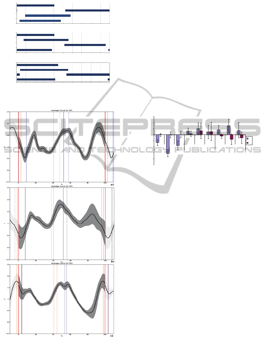
PT and RT (Figure 3). Figure 4 shows differences in

timing of events between skiers in V1 technique and

this can also be seen as differences between when

poles and skis hits/leaves ground compared to centre

of gravity total acceleration in the different skiers

(Figure 5).

MORPHOLOGICAL ANALYSIS OF ACCELERATION SIGNALS IN CROSS-COUNTRY SKIING - Information

Extraction and Technique Transitions Detection

515

FP1

0 % 10 % 20 % 30 % 40 % 50 % 60 % 70 % 80 % 90 % 100 %

right pole

right ski

left ski

left pole

FP2

0 % 10 % 20 % 30 % 40 % 50 % 60 % 70 % 80 % 90 % 100 %

right pole

right ski

left ski

left p ole

FP3

0 % 10 % 20 % 30 % 40 % 50 % 60 % 70 % 80 % 90 % 100 %

right pole

right ski

left ski

left p ole

Figure 4: Cycle phase structure in V1 for the different

subjects.

Figure 5: Average total acceleration from ACG during V1

technique. Time points for hits (solid lines) and leaves

(dashed lines) of poles (orange = right, red = left) and skis

(blue = right, purple = left), for FP1, FP2 and FP3 subjects

(Figure 5 a), b) and c) respectively).

5.3.3 Symmetry between Right

and Left Side

FP1 had clear differences in symmetry between left

and right pole in V1 compared to V2. This was not

found in the other subjects, at least not in FP2

(Figure 6). Remark that FP1 used V1r (pole push

simultaneous with right ski push) while FP2 and FP3

used V1l (pole push simultaneous with left ski

push). FP1 did not ski the end of the track where

there was a typically V1 uphill and the uphill he

(and the others) skied was in a slightly right curve.

Even though this might influence the data a bit, we

also see that FP1 has less variation (smaller standard

deviation) than the others indicating a more stable

technique (Figure 6).

-100

-80

-60

-40

-20

diff hit diff

leave

diff pt diff hit diff

leave

diff pt diff hit diff

leave

diff pt

FP1 FP2 FP3

Time (ms)

Figure 6: Time differences (Mean (SD)) in pole hit, pole

leave and PT between left and right poles. Negative values

for FP1 V1 mean that left pole hits the ground first, leaves

the ground first and right pole has most time in the ground.

6 DISCUSSION

Our approach gave good results in the detection of

pole hits/leaves and ski leaves. In addition to

calculate CT, PT and RT previously only calculated

when measuring forces (Stöggl 2010, Lindinger

2009), we were able to detect technique transitions.

Ski hits were more difficult to detect, especially

in V2 because two hits sometimes showed up. This

second hit results from a re-direction of the ski

before the push off. Some skiers clearly use this

newly developed “double-push” technique

described by Stöggl (2008), and others (like our

subjects) change technique over time using

something in between of “double-push” and

traditional V2. As the signals sometimes shows the

second hit and other times doesn’t, and we are

unsure if and when the second hit should be there

and not, the worst results we get from the ski hits

could be understood. This was also the reason why

we did not present CT, PT and RT from the skis. We

clearly have to either find a better approach or use

strain gauges or pressure sensors for detecting ski

BIOSIGNALS 2011 - International Conference on Bio-inspired Systems and Signal Processing

516

hits. One approach might be to create a separate

algorithm when the technique is classified as V2.

In addition to forces, strain gauges and force

sensors can give the same timing parameters of hits

and leaves as we have found with accelerometers,

but we will point that the weight of equipment used

for measuring forces are 3-5 times as high as our

accelerometer equipment (1,5 kg vs. 300-500g.

Stöggl 2010). We also think our equipment is easier

to put on the skiers and the skiers can use their own

poles. Even though we used accelerometers with

cables into the wireless acquisition system in this

study, there will shortly be devices available without

need of cables. This will make the preparation even

easier.

Combining different technologies like Supej

(2010) have done in alpine skiing will probably be

the future of biomechanical research. Accelerometer

data from the area around centre of gravity or

different limbs of the body in addition to force and

positioning data will probably be useful during XC-

skiing research.

7 CONCLUSIONS

Accelerometers were shown to be useful tools in XC

skiing research. Accelerometers will probably be

used more frequently in the future, in combination

with force and positioning systems. Working with

accelerometers can give insight in biological

movement patterns and can give both solutions and

ideas for more advanced biomechanical questions in

the future.

8 FUTURE WORK

The thresholds used were fitted for these subjects

and situation. Shortly, we will test the procedure on

more data and different situations. We will try to

improve our methods by finding the thresholds

automatically and we will also check what

information we can get from fewer accelerometers.

The problems of finding ski hits obviously need

more effort and we will continuously give feedback

to the producers for developing even better

equipment.

ACKNOWLEDGEMENTS

Thanks to the organising committee of the Holmen-

kollen 2010 World Cup for allowing our testing

between the arrangement, and the subjects for

participating on such short notice!

REFERENCES

Andersson, E., Supej, M., Sandbakk, Ø., Sperlich, B.,

Stöggl, T., Holmberg, H. C., 2010. Analysis of sprint

cross-country skiing using a differential global

navigation satellite system. Eur J Appl Physiol. 2010

Jun 23 (Epub ahead of print)

Holmberg, H. C., Lindinger, S., Stöggl, T., Eitzlmair, E.,

Müller, E., 2005. Biomechanical analysis of double

poling in elite cross-country skiers. MedSci in Spors &

Exercise, 37(5), 807-18.

Lindinger, S. J., Göpfert, C., Stöggl, T., Müller, E.,

Holmberg, H. C., 2009. Biomechanical pole and leg

characteristics during uphill diagonal roller skiing.

Sports Biomechanics, 8(4), pp 318-333.

Millet, G. Y., Hoffman, M. D., Vandau, R. B., Clifford, P.

S., 1998. Poling forces during roller skiing: effects of

technique and speed. Med Sci in Sports &

Exercise,30(11) pp 1645-1653.

PLUX – Wireless Biosignals, bioPLUX Research Manual,

PLUX’s internal report, 2010.

Stöggl, T., Müller, E., Lindinger, S., 2008. Biomechanical

comparison of the double-push technique and the

conventional skate skiing technique in cross-country

sprint skiing. J Sports Sci. 26(11), 1225-1233

Stöggl, T., Müller, E., Ainegren, M., Holmberg, H. C.,

2010. General strength and kinetics: fundamental to

sprinting faster in cross country skiing? Scand J Med

Sci Sports, 2010, 1-13.

Supej, M. 2010. 3D measurements of alpine skiing with an

inerial sensor motion capture suit and GNSS RTK

system. J Sports Sci. 28(7), 759-69.

T. Oliphant. Guide to Numpy. Tregol Publishing, 2006.

T. Oliphant. SciPy Tutorial. SciPy, http://www.scipy.

org/SciPy Tutorial, 2007.

www.dartfish.com, 2010, last accessed on 19/07/2010

MORPHOLOGICAL ANALYSIS OF ACCELERATION SIGNALS IN CROSS-COUNTRY SKIING - Information

Extraction and Technique Transitions Detection

517