OPTICAL FLOW BY MULTI-SCALE ANNOTATED KEYPOINTS

A Biological Approach

Miguel Farrajota, J. M. F. Rodrigues and J. M. H. du Buf

Vision Laboratory, Institute for Systems and Robotics (ISR)

University of the Algarve (ISE and FCT), 8005-139 Faro, Portugal

eywords:

Optical ﬂow, Multi-scale, Keypoint classiﬁcation, Visual cortex, Segregation, Tracking.

Abstract:

Optical ﬂowis the pattern of apparent motion of objects in a visual scene and the relative motion, or egomotion,

of the observer in the scene. In this paper we present a new cortical model for optical ﬂow. This model is based

on simple, complex and end-stopped cells. Responses of end-stopped cells serve to detect keypoints and those

of simple cells are used to detect orientations of underlying structures and to classify the junction type. By

combining a hierarchical, multi-scale tree structure and saliency maps, moving objects can be segregated, their

movement can be obtained, and they can be tracked over time. We also show that optical ﬂow at coarse scales

sufﬁces to determine egomotion. The model is discussed in the context of an integrated cortical architecture

which includes disparity in stereo vision.

1 INTRODUCTION

Optical ﬂow, also called optic ﬂow, is the motion pat-

tern caused by moving objects in a visual scene. It

can be described by motion or displacement vectors

of entire objects or parts of them between successive

time frames. In the case of egomotion, i.e., the eye

of a moving person or a moving camera, the relative

motion between observer and scene also contributes.

Experiments have strengthened the arguments that

neurons in a specialised region of the cerebral cortex

play a major role in ﬂow analysis (Wurtz, 1998), that

neuronal responses to ﬂow are shaped by visual strate-

gies for steering (William and Charles, 2008), and

that ﬂow processing has an important role in the de-

tection and estimation of scene-relative object move-

ments during egomotion (Warren and Rushton, 2009).

For the latter, the brain identiﬁes and globally dis-

counts (i.e., subtracts) optical ﬂow patterns across the

visual scene, a process called ﬂow parsing.

(Morrone et al., 2000) demonstrated that neurons

in area V5/MT (medial temporal) respond selectively

to components of optical ﬂow, such as circular and

radial motion. (Smith et al., 2006) showed that neu-

rons in area MST (middle superior temporal) seem to

be more selective to complex movements than those

in area MT, the latter being more devoted to simple

movements, although both areas respond to all mo-

tion stimuli but with different activation patterns. Al-

though many cells may respond to more than one type

of motion stimulus, individual cells show different di-

rection selectivities (Duffy and Wurtz, 1991). In ad-

dition, cells in area MST were reported to be selective

for rotation and expansion (Orban et al., 1992), hav-

ing larger receptive ﬁelds and less precise retinotopic

mapping than those in area MT. Therefore, MST cells

conveymore global information about a scene’s struc-

ture and motions (Smith et al., 2006).

An essential function of visual processing is to

establish the position of the body in space and, in

concert with the other sensory systems, to monitor

its movements: egomotion through optical ﬂow (Wall

and Smith, 2008). For example, forward motion gen-

erates an expanding ﬂow pattern on the retinae and,

with eyes ﬁxated centrally, the heading direction cor-

responds to the centre of expansion. Area MST being

sensitive to more global optical ﬂow patterns, it has

been suggested that MST has a central role in guid-

ing heading in macaques. The same authors identi-

ﬁed two areas of the human brain which represent vi-

sual cues to egomotion more directly than does area

MST. One is the putative area VIP in the anterior part

of the intraparietal sulcus. The other is a new visual

area coined cingulate sulcus visual area (CSv). In

contrast to these new areas, areas V1 to V4 and MT

respond about equally to stimuli mimicking arbitrary

motion and egomotion, whereas area MST has inter-

mediate properties, responding well to various motion

307

Farrajota M., M. F. Rodrigues J. and M. H. du Buf J..

OPTICAL FLOW BY MULTI-SCALE ANNOTATED KEYPOINTS - A Biological Approach.

DOI: 10.5220/0003172403070315

In Proceedings of the International Conference on Bio-inspired Systems and Signal Processing (BIOSIGNALS-2011), pages 307-315

ISBN: 978-989-8425-35-5

 2011 SCITEPRESS (Science and Technology Publications, Lda.)

stimuli but with a modest preference for egomotion-

compatible stimuli.

Apart from motion processing, we know that the

visual cortex detects and recognises objects by means

of the ventral “what” and dorsal “where” subsystems.

Both bottom-up (visual input code) and top-down(ex-

pected object and position) data streams are necessary

for obtaining size, rotation and translation invariance,

assuming that object templates are normalised in vi-

sual memory.

Recently we presented cortical models based on

multi-scale line/edge and keypoint representations

(Rodrigues and du Buf, 2006; Rodrigues and du Buf,

2009b). These representations, all based on responses

of simple, complex and end-stopped cells in V1, can

be integrated for different processes: visual recon-

struction or brightness perception, focus-of-attention

(FoA), object segregation and categorisation, and ob-

ject and face recognition. The integration of FoA, re-

gion segregation and object categorisation is impor-

tant for developing fast gist vision, i.e., which types

of objects are about where in a scene.

Optical ﬂow, as for disparity in stereo vision, com-

plements colour and texture in object segregation,

possibly in, but not necessarily limited to, the dorsal

“where” pathway where keypoints may play a major

role in FoA (Rodrigues and du Buf, 2006). In this pa-

per we present a new model for cortical optical ﬂow

which is based on annotated (classiﬁed) multi-scale

keypoints. We show that the information can be used

for egomotion and for object segregation and track-

ing.

In Section 2 we present multi-scale keypoint de-

tection and annotation, in Section 3 optical ﬂow de-

tection, in Section 4 object tracking using optical ﬂow

information, and we conclude with a ﬁnal discussion

and lines for future work in Section 5.

2 MULTI-SCALE KEYPOINT

ANNOTATION

Keypoints are based on end-stopped cells (Rodrigues

and du Buf, 2006). They provide important informa-

tion because they code local image complexity. More-

over, since keypoints are caused by line and edge jun-

tions, detected keypoints can be classiﬁed by the un-

derlying vertex structure, such as K, L, T, + etc. This

is very useful for most if not all matching problems:

object recognition, stereo disparity and optical ﬂow.

In this section we describe the multi-scale keypoint

detection and annotation processes.

2.1 Keypoint Detection

Gabor quadrature ﬁlters provide a model of cortical

simple cells (Rodrigues and du Buf, 2006). In the

spatial domain (x,y) they consist of a real cosine and

an imaginary sine, both with a Gaussian envelope.

Responses of even and odd simple cells, which cor-

respond to real and imaginary parts of a Gabor ﬁl-

ter, are obtained by convolving the input image with

the ﬁlter kernel, and are denoted by R

s,i

(x,y) and

s,i

(x,y), s being the scale, i the orientation (θ

iπ/N

) and N

the number of orientations (here 8)

with i = [0,N

− 1]. Responses of complex cells are

then modelled by the modulus

s,i

(x,y) = [{R

s,i

(x,y)}

+ {R

s,i

(x,y)}

]

1/2

There are two types of end-stopped cells, single and

double. These are applied to C

s,i

and are combined

with tangential and radial inhibition schemes in or-

der to obtain precise keypoint maps K

(x,y). For a

detailed explanation with illustrations see (Rodrigues

and du Buf, 2006). Below, the scale of analysis will

be given by λ expressed in pixels, where λ = 1 corre-

sponds to 1 pixel.

Figure 1 (top-left) shows a scene with, on the sec-

ond row from top, keypoints detected (diamond sym-

bols) at two scales λ = 6 (left) and 27 (right). At

top-right it shows one quadrant of a test image with

a black square against a homogeneous background

(top-left) and a noisy background (top-right), both

with a correctly detected keypoint at the junction. All

other images show annotated keypoints; see below.

2.2 Keypoint Annotation

In order to classify any detected keypoint, the re-

sponses of simple cells R

s,i

and R

s,i

are analysed, but

now using N

= 2N

orientations, φ

= kπ/N

and

k = [0, N

− 1]. This means that for each simple-

cell orientation on [0,π] there are two opposite anal-

ysis orientations on [0,2π], e.g., θ

= π/N

results in

= π/N

and φ

= 9π/N

; see Fig. 2 (top).

This division into response-analysis orientations

is acceptable, according to (Hubel, 1995), because a

typical cell has a maximum response at some orienta-

tion and its response decreases on both sides, from 10

to 20 degrees, after which it declines steeply to zero;

see also (du Buf, 1993). In addition, this division is a

compromise between the cost (CPU time) of the num-

ber of orientations and the accuracy of the results.

Classifying keypoints is not trivial, because re-

sponses of simple and complex cells, which code the

underlying lines and edges at the vertices, are unre-

liable due to response interference effects (du Buf,

BIOSIGNALS 2011 - International Conference on Bio-inspired Systems and Signal Processing

308

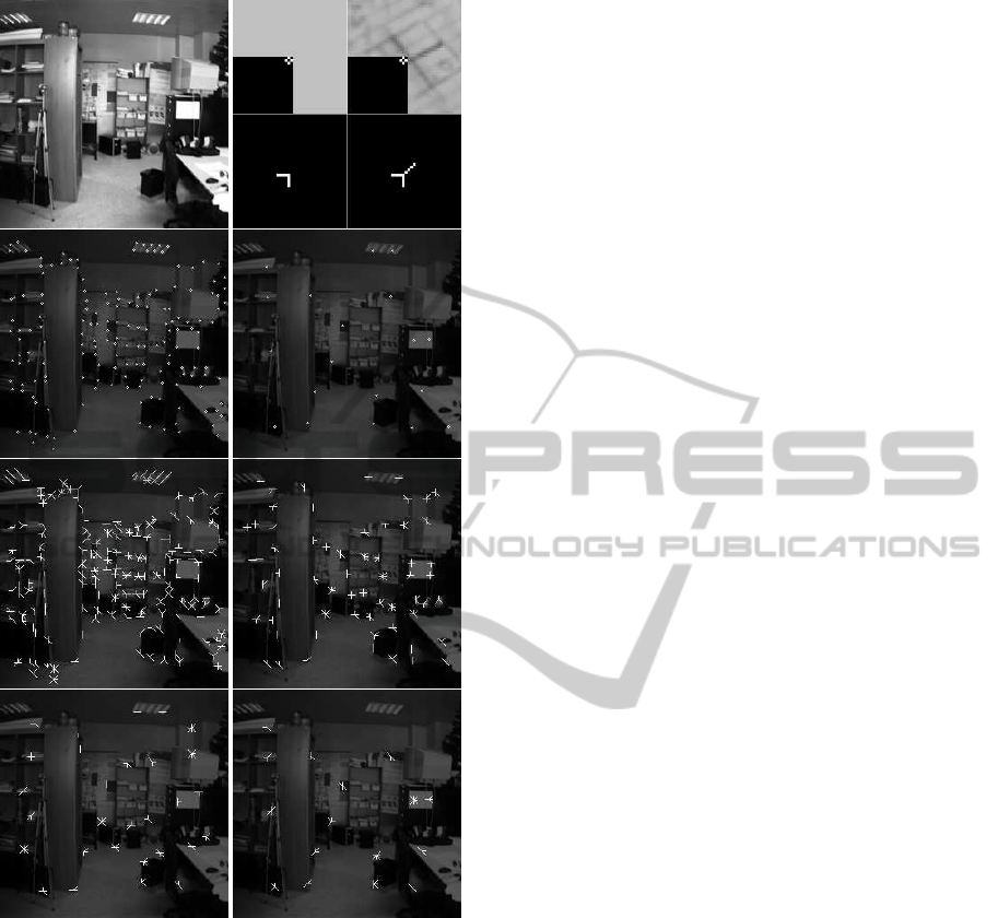
Figure 1: Keypoint detection and annotation. Input scene

(top-left) with, on the 2nd row, keypoints detected at scales

λ = 6 (left) and 27 (right). The 3rd and 4th rows show anno-

tated keypoints at scales λ = {6, 12,18,27}. The top-right

image shows one quadrant of a black square against a ho-

mogeneous background (left) and noisy background (right),

both at λ = 6.

1993). This implies that responses must be analysed

in a neighbourhood around each keypoint, and the

size of the neighbourhood must be proportional to the

scale of the cells. The validation of the line and edge

orientations which contribute to the vertex structure is

based on an analysis of the responses of simple cells,

both R

s, j

and R

s, j

, and consists of three steps: (1) only

responses with small variations at three distances are

considered, (2) local maxima of the responses over

orientations are probed and the remaining orientations

are inhibited, and (3) responses of even and odd sim-

ple cells are matched in order to keep the orientations

which are common to both.

In step (1), at any scale and each orientation φ

the

responses of the simple cells on three circles around

the keypoint position, with radii λ/2, λ and 2λ, are

compared. Instead of only taking the responses at

, the orientation intervals φ

± π/N

are considered.

The three maximum responses of R

E/O

k,r

in the orien-

tation interval around k and at the three radii r are

detected, and their maximum

= max

E/O

k,r

. Only

responses with small variations at the three radii are

considered (R > 0.6

), yielding N

candidate ori-

entations. The smallest radius of λ/2 was chosen

because of the interference effects referred to above

(du Buf, 1993). The other two radii were determined

experimentally.

Biologically, the above process is based on clus-

ters of groupingcells with dendritic ﬁelds (Fig. 2 (top)

in red) covering the orientation intervals at each of

the three radii. These grouping cells combine other

cells with self-inhibition for non-maximum suppres-

sion. The three grouping cells at the three radii feed

into another grouping cell which compares the re-

sponses and which inhibits itself when the responses

are not similar. Figure 2 (bottom) shows responses

of simple cells in the case of a black square against

a noisy background (Fig. 1 top-right). It shows two

scales, λ = 6 (column 1 and 2) and λ = 15 (column 3

and 4), only three of all eight orientations (top to bot-

tom), even cells in columns 1 and 3 and odd cells in

columns 2 and 4. Dark levels are negative and bright

ones are positive. Also shown is one detected key-

point at each scale with, in red, the three circles at

λ/2, λ and 2λ at which the grouping cells are located.

The drawing at the top shows the orientation intervals,

also in red, covered by the dendritic ﬁelds in the case

of θ

with opposite orientations φ

and φ

In step (2), the responses at the detected orienta-

tions are summed,

R = Σ

, and, for validation pur-

poses, all responses

below a threshold value of

are suppressed (0.95

R/N

). Biologically, this is done

by another grouping cell which sums responses of the

grouping cells in step (1) and which may inhibit the

same cells if their response is too low.

If there also exist maximum responses

at the

two neighbouring orientations φ

k−1

and φ

k+1

, they

will be inhibited if they are too low (

k±1

< 0.95

The abovevalues were determined by analysing many

objects like triangles, squares and polygons.

Step (2) is necessary because we need the orienta-

tions which convey the most consistent information,

i.e., not being due to varying lighting levels, light

sources casting shadows, background structures and

OPTICAL FLOW BY MULTI-SCALE ANNOTATED KEYPOINTS - A Biological Approach

309

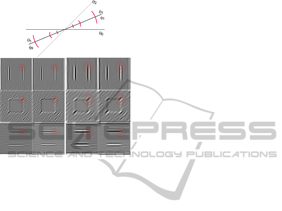
Figure 2: Top: a few orientations of simple cells (θ) and

opposing orientations for keypoint classiﬁcation (φ) plus, in

red, orientation intervals covered by grouping cells. Bot-

tom: responses of simple cells at 3 orientations (top to bot-

tom) and at two scales λ = 6 (left) and λ = 15 (right). From

left to right: responses of even and odd simple cells. Also

shown is one detected keypoint with, in red, the 3 circles on

which the responses are analysed for keypoint annotation.

even dynamic backgrounds like the wind playing the

crowns of trees. Figure 1 (top-right) shows the dif-

ference in the case of the same black square against a

homogeneous background (left) and a structured one

(right). The diagonal structure in the background has

a much lower contrast than the edge of the square.

Hence, without step (2) the keypoint would have been

annotated by three orientations instead of two.

The analysis in step (3) only concerns the match-

ing of equal orientations, i.e., inhibiting all orienta-

tions which have not been detected in the responses of

both even (R

s, j

) and odd (R

s, j

) simple cells. Remain-

ing orientations φ

are attributed to the keypoint, plus

the junction type K, L, T, +, etc. Again, the match-

ing is achieved by grouping cells which combine the

grouping cells devoted to R

s, j

and R

s, j

In the above procedure there is only one excep-

tion: keypoints at isolated points and blobs, especially

at very coarse scales, are also detected but they are not

caused by any line/edge junctions. Such keypoints are

labeled “blob” without attributed orientations.

The bottom four images in Fig. 1 show re-

sults of keypoint annotation at the four scales λ =

{6,12, 18,27}. At ﬁne scale there are many keypoints

and at coarse scale less. Below, the annotated key-

points will be exploited in different processes. As

mentioned above, keypoint detection may occur in

cortical areas V1 and V2, whereas keypoint annota-

tion requires bigger receptive ﬁelds and could occur

in V4. Optical ﬂow is then processed in areas V5/MT

and MST.

3 OPTICAL FLOW

Optical ﬂow is determined by matching annotated

keypoints in successive camera frames, but only by

matching keypoints which may belong to the same

object. To this purpose we use regions deﬁned

by saliency maps. Moreover, we do not consider

all scales independently, for two reasons: (1) non-

relevant areas of an image can be skipped because of

the hierarchical scale structure, and (2) by applying a

hierarchical tree structure, the accuracy of the match-

ing can be increased, therefore also increasing the ac-

curacy of the optical ﬂow. The latter idea is based on

the strategies as employed in our visual system (Ro-

drigues and du Buf, 2009a; Bar, 2004).

3.1 Object Segregation

We apply a multi-scale tree structure in which at a

very coarse scale a root keypoint deﬁnes a single ob-

ject, and at progressively ﬁner scales more keypoints

are added which convey the object’s details. However,

coarser scales imply bigger ﬁlter kernels and more

CPU time, so for practical reasons the coarsest scale

applied here will be λ = 27, which is a compromise

between speed and quality of results.

Below we use λ = [6,27] with ∆λ = 3, and at the

moment all keypoints at λ = 27 are supposed to rep-

resent individual objects, although we know that it is

possible that several of those keypoints may belong

to a same object. Each keypoint at a coarse scale is

related to one or more keypoints at one ﬁner scale,

which can be slightly displaced. This relation is mod-

elled by down-projection using grouping cells with

a circular axonic ﬁeld, the size of which (λ) deﬁnes

the region of inﬂuence. A responding keypoint cell

activates a grouping cell. Only if the grouping cell

is also excitated by responding keypoint cells at one

level lower (the next ﬁner scale), a grouping cell at

the lower level is activated. This is repeated until the

ﬁnest scale has been reached. By doing so, all key-

points outside the areas of inﬂuence of the grouping

cells will not be considered, thus avoiding unneces-

sary computations. Figure 3 (top) illustrates the prin-

ciple of the linking process with cones representing

BIOSIGNALS 2011 - International Conference on Bio-inspired Systems and Signal Processing

310

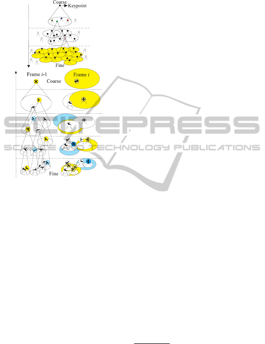
Figure 3: Top: hierarchical tree structure over scales. Bot-

tom: matching of annotated keypoints between successive

frames; see text for details.

the axonic ﬁelds of the grouping cells. At the ﬁnest

scale the region of inﬂuence of the keypoint at the

coarsest scale is indicated by the yellow area.

As mentioned above, at a very coarse scale each

keypoint – or central keypoint CKP – should corre-

spond to an individual object. However, at the coars-

est scale applied, λ = 27, this may not be the case and

an object may cause several keypoints. In order to

determine which keypoints could belong to the same

object we combine saliency maps with the multi-scale

tree structure.

A saliency map can be based on keypoints as these

code local image complexity (Rodrigues and du Buf,

2006). Such a map is created by summing detected

keypoints over all scales s, such that keypoints which

are stable over scale intervals yield high peaks, but

in order to connect the individual peaks and yield re-

gions a relaxation area is applied. As applied above,

the area is proportional to the scale and has a ra-

dius of λ. Here, we simplify the computation of

saliency maps by summing responses of end-stopped

cells at all scales, which yields similar results. Fig-

ure 6 (right) shows on the 2nd to the 4th row examples

of such saliency maps which correspond to the input

frames to their left. For illustration purposes the maps

were scaled to the interval [0,255]. The maps will be

thresholded in order to obtain segregated regions; see

below.

3.2 Keypoint Matching

At this point we have, for each frame, the tree struc-

ture which links the keypoints over scales, from

coarse to ﬁne, with associated regions of inﬂuence

at the ﬁnest scale. We also have the saliency map

by summing responses of end-stopped cells over all

scales. The latter, after thresholding, yields segre-

gated regions which are intersected with the regions

of inﬂuence of the tree. Therefore, the intersected re-

gions link keypoints at the ﬁnest scale to segregated

regions which are supposed to represent individual

objects.

Now, each annotated keypoint of frame i can be

compared with all annotated keypoints in frame i− 1.

This is done at all scales, but the comparison is re-

stricted to an area with radius 2λ instead of λ at each

scale in order to allow for larger translations and ro-

tations. In addition: (1) at ﬁne scales many keypoints

outside the area can be skipped since they are not

likely to match over large distances, and (2) at coarse

scales there are less keypoints, λ is bigger and there-

fore larger distances (motions) are represented there.

The tree structure is built top-down, Fig. 3 (top), but

the matching process, Fig. 3 (bottom), is bottom-up:

it starts at the ﬁnest scale because there the accuracy

of the keypoint annotation is better. Keypoints are

matched by combining three similarity criteria with

different weight factors: the distance D, the attributed

orientations O, and the tree correspondence C.

The distance D serves to emphasise keypoints

which are closer to the centre of the matching area.

For having D = 1 at the centre and D = 0 at radius

2λ, we use D = (2λ − d)/2λ with d the Euclidean

distance. Biologically, there may be no need to use

Euclidean distances if a kind of dynamic feature rout-

ing in space and time is used, possibly with motion

prediction in the “where” pathway.

Dynamic routing

from frame i − 1 to frame i, possibly also involving

previous frames i − 2 etc., is a spatiotemporal map-

ping, assuming a stack of neural layers in which a

few previous maps are stored: a new frame is al-

ways pushed on the “top-of-stack” and older frames

are also being pushed down. As for dynamic rout-

ing in invariantobject recognition, see (Rodriguesand

Motion prediction is a form of adaptation which could

explain the motion aftereffect, for example our illusion that

a railway station moves after our train has stopped. This

may occur in area MT (Kohn and Movshon, 2003).

OPTICAL FLOW BY MULTI-SCALE ANNOTATED KEYPOINTS - A Biological Approach

311

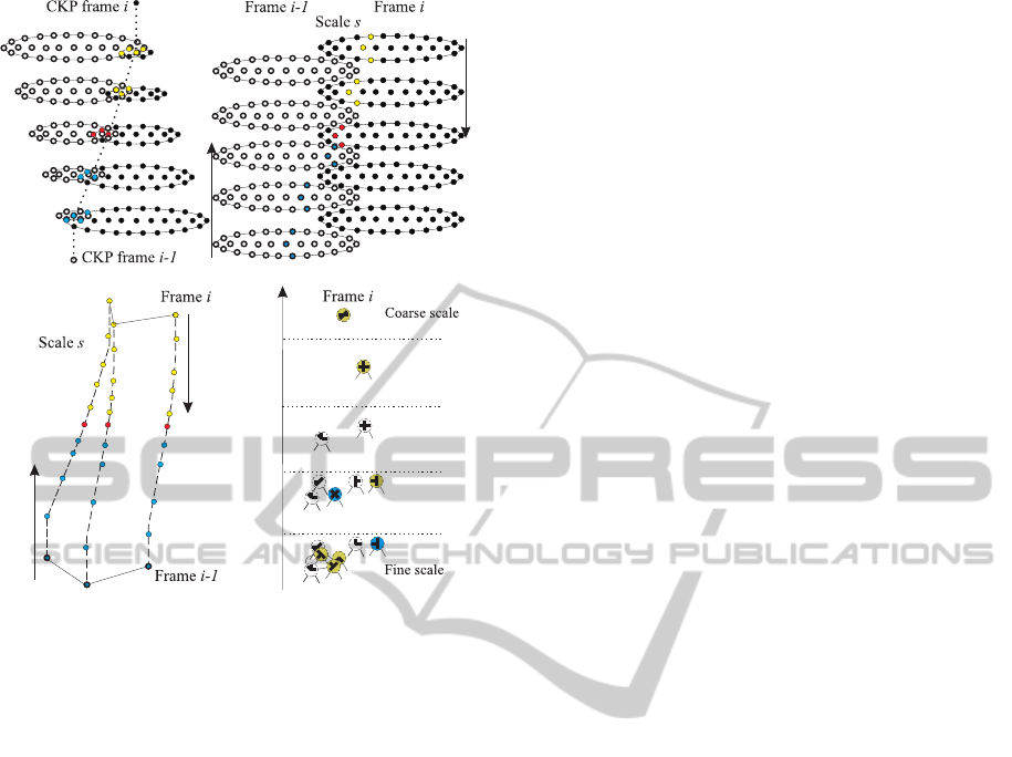
Figure 4: Top: dynamic routing between coarse keypoints

of successive frames (left), and cell representation of dis-

tance D (right). Bottom: cell representation of orientation

O (left), and tree correspondence C (right); see text for de-

tails.

du Buf, 2009a), the principle can be based on linking

ﬁrst keypoints at very coarse scales (central keypoints

or CKP in Fig. 4 top-left) in space after which ﬁner

scales reﬁne the linking (Fig. 4 top-right). This is sub-

ject to ongoing research.

The orientation error O measures the differences

of the attributed orientations, but with a relaxation of

±π/N

of all orientations such that also a small ro-

tation of the vertex structure is allowed. Similar to

D, the summed differences are combined such that

O = 1 indicates good correspondence and O = 0 a

lack of correspondence. Obviously, keypoints marked

“blob” do not have orientations and are treated sep-

arately. Biologically, the orientation error could be

based on the number of intermediate layers in the

routing which is necessary to establish correspon-

dence of the vertex structure, which is shown simpli-

ﬁed in Fig. 4 (bottom-left).

Parameter C measures the number of matched

keypoints at ﬁner scales, i.e., at any scale coarser than

the ﬁnest one. The keypoint candidates to be matched

in frame i and in the area with radius 2λ are linked

in the tree to localised sets of keypoints at all ﬁner

scales. The number of linked keypoints which have

been matched is divided by the total number of linked

keypoints. This is achieved by sets of grouping cells

at all but the ﬁnest scale which sum the number of

linked keypoints in the tree, both matched and all.

Hence, parameter C describes the consistency of the

matching at a candidate’s position at the ﬁner scales,

thereby inﬂuencing the matching of the candidate at

the actual scale. Figure 4 (bottom-right) illustrates

in colour the matched keypoints which inﬂuence the

matching at coarser scales; see also Fig. 3 (bottom).

The three parameters are combined by grouping

cells which can establish a link between keypoints in

frame i− 1 and i. Mathematically we use the similar-

ity measure S = αO+ βC+ γD, with α = 0.4, β = 0.3

and γ = 0.3. These values were determined empiri-

cally. The candidate keypoint with the highest value

of S in the area (2λ) is selected and the vector between

the keypoint in frame i − 1 and the matched one in

frame i is computed. The remaining candidates in the

area can be matched to other keypoints in frame i− 1,

provided they are in their local area. Keypoints which

cannot be matched are discarded.

Figure 5 (top-left) shows a sequence of 10 frames

with a moving and rotating star combined into one

image and, at right, examples of keypoints detected at

scales λ = 6 (left) and 24 (right), together with their

annotation below. The 2nd row (left) shows the opti-

cal ﬂow vectors from the ﬁrst to the last frame. The

other images show two superimposed frames with

egomotion of the camera and the optical ﬂow vectors

at four scales λ = {6, 12,18,27}. It can be seen that

there are some but few errors. In principle, such out-

liers can be removed, but important is that the cor-

rect egomotion can be seen at all scales with, as ex-

pected, more variation at the ﬁnest scale. In fact, the

ﬂow detected at the coarsest scale (bottom-right) is

already sufﬁcient to extract the egomotion. This is

consistent with object categorisation and recognition

(Bar, 2004; Oliva and Torralba, 2006; Rodrigues and

du Buf, 2009b): coarse-scale information is available

ﬁrst and this is used for a ﬁrst but rough categorisation

(80 – 100 ms), after which information at ﬁner scales

becomes available to reﬁne the categorisation.

After obtaining egomotion vectors at the coarsest

scale, by averaging but perhaps after elimination of

outliers in local neighbourhoods because of possible

camera rotation, egomotion can be eliminated by sub-

tracting this information from all ﬂow vectors (War-

ren and Rushton, 2009). Bearing this in mind, when

we compute the tree correspondence C for keypoint

matching at only the coarsest scale, the result will be

similar. However, the result will be more robust if

we use all scales, as in the object categorisation and

recognition process (Rodrigues and du Buf, 2009b).

BIOSIGNALS 2011 - International Conference on Bio-inspired Systems and Signal Processing

312

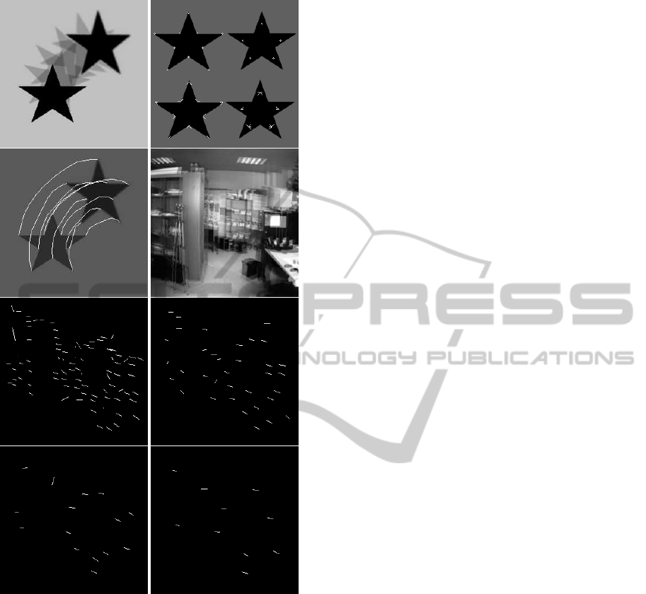
Figure 5: Optical ﬂow results. Top-left: frames with a mov-

ing and rotating star combined into one image. Top-right:

detected keypoints at scales λ = 6 (left) and 24 (right), with

the annotated keypoints below. Second from top, at left, op-

tical ﬂow vectors. The other images show two combined

frames with egomotion of the camera and optical ﬂow vec-

tors at scales λ = {6,12,18,27}.

4 TRACKING OF OBJECTS

After thresholding, the saliency map of a frame yields

separated regions-of-interest(RoI); see Fig. 6, the 2nd

to 4th row at right. These regions can be intersected

with the regions as deﬁned by the tree structure, in

Fig. 3 (top) shown in yellow. The regions of the den-

dritic ﬁelds of the end-stopped cells which generate

the saliency map will overlap the regions of the ax-

onic ﬁelds of the keypoint-grouping cells in the tree

structure. Hence, neighbouring keypointsare grouped

together in the RoIs and their displacement vectors

after the matching process yield the optical ﬂow of

segregated image regions, i.e., where an individual

object or a combination of connected (sub)objects is

or are moving. In order to discard very small opti-

cal ﬂow due to the camera’s motion (not signiﬁcant

egomotion; see above) and to obtain more robust re-

sults, optical ﬂow vectors are only computed if at at

least four scales the matched keypoints in successive

frames have displacement vectors with a length which

is bigger than one pixel.

Figure 6 (top) shows a montage of a sequence with

a moving robot car (at left) and the tracked optical

ﬂow vectors (at right): in white for λ = 6 and in red

for λ = 27. Rows 2 to 4 show frames with the robot

car segregated in a box (at left) and the correspond-

ing saliency maps (at right). The bottom row shows

zooms of two frames with ﬂow vectors at scale λ = 9.

Figure 7 shows two more sequences with moving

persons. The top sequence shows a moving person far

away, with the bounding box and tracked motion (ar-

rows). The bottom sequence shows a person at close

range, in which case the different motions of the dif-

ferent body parts can be distinguished, also the mo-

tion of the shadow. The bottom sequence illustrates

a real application: detecting and tracking moving ob-

stacles on paths and sidewalks, which is for a naviga-

tion aid for the blind in the context of the SmartVision

project. In this case the optical ﬂow is complemented

by the borders of the path and their intersection in the

vanishing point, and the tracking of the centre of the

bounding box relative to the vanishing point can be

used to detect if the obstacle is approaching or not,

for obstacle avoidence.

5 CONCLUSIONS

In a previous paper we have shown that keypoint

scale-space provides very useful information for con-

structing saliency maps for Focus-of-Attention(FoA),

and that faces can be detected by grouping facial land-

marks deﬁned by keypoints at eyes, nose and mouth

(Rodrigues and du Buf, 2006). We have also shown

that line/edge scale-space provides very useful infor-

mation for face and object recognition (Rodrigues

and du Buf, 2009b). Obviously, object detection and

recognition are related processes, with a seamless in-

tegration in the where and what pathways. However,

there is no (known) dichotomy in the sense that key-

points are only used in the where pathway and lines

OPTICAL FLOW BY MULTI-SCALE ANNOTATED KEYPOINTS - A Biological Approach

313

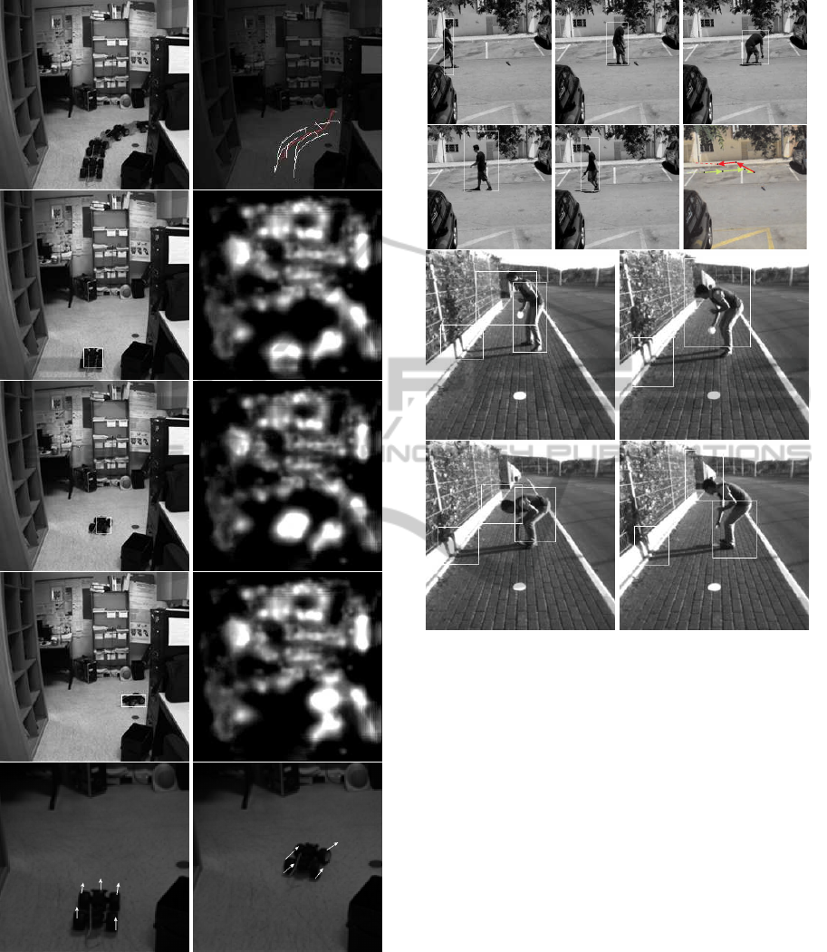
Figure 6: Top: a sequence with a moving robot car (left)

and combined optical ﬂow vectors (right), in white at a ﬁne

scale and in red at a coarse scale. Rows 2 to 4 show frames

with the robot car segregated in a box (left) and the cor-

responding saliency maps (right). The bottom row shows

zooms of optical ﬂow vectors at scale λ = 9.

and edges only in the what pathway.

In this paper we showed that keypoint detection

Figure 7: Two sequences with moving persons. The per-

sons have been segregated (bounding box) and tracked (top

sequence; arrows), and differently moving body parts have

been detected, including shadows (bottom sequence).

can be complemented by keypoint annotation, and

that annotated keypoints in a hierarchical tree struc-

ture can be used for keypoint matching in order to

obtain optical ﬂow. In addition, since local clusters

of keypoints are mostly related to individual moving

objects, object segregation can be achieved and ob-

jects can be tracked. As written before, cortical areas

MT and MST are involved in optical ﬂow and egomo-

tion, but recent results obtained with fMRI showed no

clear neural activity in their ventral (what) and dor-

sal (where) subregions, but elevated activity in be-

tween the subregions (Smith et al., 2006). This might

indicate that optical ﬂow at MT level is processed

separately or involves both pathways. The fact that

optical ﬂow can be used to obtain object segrega-

tion, as demonstrated here, in addition to our previous

experiments concerning saliency maps for FoA and

face detection, in all cases only using keypoint scale

space, would indicate some “preference” of the dorsal

BIOSIGNALS 2011 - International Conference on Bio-inspired Systems and Signal Processing

314

(where) pathway for keypoints. This idea is strength-

ened by the fact that area MT also plays a role in

the motion-aftereffect illusion (Kohn and Movshon,

2003), which is tightly related to motion adaptation

and prediction. Therefore, motion prediction might

play a very important role in the dorsal pathway, not

only where objects are now but also where they are

expected next. Such predictions tied to objects may

lead to much more efﬁcient processing, for exam-

ple in robot vision, because most image regions can

be skipped. Nevertheless, robot vision also requires

some sort of “arousal” system for spotting new or un-

expected moving objects.

Having a model for matching keypoints in con-

secutive time frames for optical ﬂow, the same prin-

ciple can be applied to stereo (disparity), matching

left and right frames. Since information of one of the

two frames is already available for optical ﬂow, the re-

quired additional CPU time will be limited, especially

if only the distance of moving objects is necessary, for

example to detect objects which may be on collision

course, with and without egomotion. In general, how-

ever, disparity can be used for obtaining a 3D sketch

of an entire scene, plus the 3D structure of individual

objects in the scene which may complement the (2D)

line/edge scale space for object recognition. More-

over, optical ﬂow and disparity can be combined to

obtain more robust object segregations.

Keypoints can complement the line/edge coding

in attributing depth, not only to vertical lines and

edges but also line and edge junctions. This results

in a sort of 3D “wireframe” representation as used in

modelling solid objects in computer graphics. The

fact that projections from left and right eyes are very

close in the cortical hypercolumns and that many sim-

ple and complex cells are also disparity tuned sug-

gests that our visual system processes 3D objects in

the same way, probably simplifying 3D object recog-

nition.

ACKNOWLEDGEMENTS

Portuguese Foundation for Science and Technol-

ogy (FCT) through the pluri-annual funding of

the Inst. for Systems and Robotics (ISR/IST), the

POS Conhecimento Program with FEDER funds, and

FCT project SmartVision (PTDC/EIA/73633/2006).

REFERENCES

Bar, M. (2004). Visual objects in context. Nature Rev.:

Neuroscience, 5:619–629.

du Buf, J. (1993). Responses of simple cells: events, inter-

ferences, and ambiguities. Biol. Cybern., 68:321–333.

Duffy, C. and Wurtz, R. (1991). Sensitivity of mst neu-

rons to optic ﬂow stimuli. I. A continuum of response

selectivity to large-ﬁeld stimuli. J. Neurophysiol.,

65(6):1329–1345.

Hubel, D. (1995). Eye, Brain and Vision. Scientiﬁc Ameri-

can Library.

Kohn, A. and Movshon, J. (2003). Neuronal adaptation to

visual motion in area mt of the macaque. Neuron,

39:681–691.

Morrone, M., Tosetti, M., Montanaro, D., Fiorentini, A.,

Cioni, G., and Burr, D. (2000). A cortical area that

responds speciﬁcally to optic ﬂow, revealed by fMRI.

Nature Neuroscience, 3(7):1322 – 1328.

Oliva, A. and Torralba, A. (2006). Building the gist of a

scene: the role of global image features in recognition.

Progress in Brain Res.: Visual Perception, 155:23–26.

Orban, G., Lagae, L., Verri, A., Raiguel, S., Xiao, D., Maes,

H., and Torre, V. (1992). First-order analysis of optical

ﬂow in monkey brain. PNAS, 89(7):2595–2599.

Rodrigues, J. and du Buf, J. (2006). Multi-scale keypoints

in V1 and beyond: object segregation, scale selection,

saliency maps and face detection. BioSystems, 2:75–

90.

Rodrigues, J. and du Buf, J. (2009a). A cortical frame-

work for invariant object categorization and recogni-

tion. Cognitive Processing, 10(3):243–261.

Rodrigues, J. and du Buf, J. (2009b). Multi-scale lines and

edges in v1 and beyond: brightness, object categoriza-

tion and recognition, and consciousness. BioSystems,

95:206–226.

Smith, A., Wall, M., Williams, A., and Singh, K. (2006).

Sensitivity to optic ﬂow in human cortical areas

mt and mst. European Journal of Neuroscience,

23(2):561–569.

Wall, M. and Smith, A. (2008). The representation of ego-

motion in the human brain. Current Biology, 18:191–

194.

Warren, P. and Rushton, S. (2009). Optic ﬂow process-

ing for the assessment of object movement during ego

movement. Current Biology, 19(19):1555–1560.

William, K. and Charles, J. (2008). Cortical neuronal re-

sponses to optic ﬂow are shaped by visual strategies

for steering. Cerebral Cortex, 18(4):727–739.

Wurtz, R. (1998). Optic ﬂow: A brain region devoted to

optic ﬂow analysis? Current Biology, 8(16):R554–

R556.

OPTICAL FLOW BY MULTI-SCALE ANNOTATED KEYPOINTS - A Biological Approach

315