LITTER EFFECT IN MOUSE PHENOTYPIC STUDIES
Petr Simecek, Maria Dzur-Gejdosova, Irena Chvatalova and Jiri Forejt
Institute of Molecular Genetics of the ASCR and Center for Applied Genomics, Vídeňská 1083, Prague, Czech Republic
Keywords: Litter effect, Mixed-effect models, Phenome databases, Mouse genetics.
Abstract: The laboratory mouse is the most common mammalian model organism for research of the human body
functions and disorders. For experimental purposes mice selected from inbred strains, developed by many
generations of brother-sister crosses, are usually used. Individual mice of a given inbred strain are therefore
considered genetically identical. However, our preliminary observations suggest that for a number of
phenotypic traits mice originating from the same litter are significantly more similar than mice coming from
different litters of the same inbred strain. We estimated the size of this litter effect for a number of traits in
several phenotypic studies. By means of simulation we showed that ignoring the litter effect may result in
several fold higher false positive rate and severe underestimation of minimal sample size.
1 INTRODUCTION
Starting with the work of Gregor Mendel, genetics
has always been one of more mathematically
oriented areas of biology. As time goes by, the
geneticists adopted various statistical tools: from
Student’s T-test through Wright’s path analysis and
Fisher’s work on Mendelian inheritance to modern
robust and Bayesian methods for processing the
microarrays.
Statistical methods, even the simplest ones, are
always based on a number of assumptions. It is
important to know about them and to know about
consequences of their infringement. In real life
variances are often heterogeneous, measurements
not independent and distributions far from the ideal
Gaussian bell shaped curve. Dealing with these
issues is crucial and there is a vast amount of
literature how ignoring the unstated assumptions can
lead to false conclusions, eg. (Glass et al., 1972).
This paper is focused on a very concrete issue in
the field of mouse genetics – a litter effect (LE) in
phenotyping studies, particularly in large scale
phenotyping studies. For genetic analyses we usually
use mouse inbred strains, developed by many
generations of brother-sister crosses (Silver, 1995,
p. 32). Individual mice of the same inbred strain are
therefore considered genetically identical.
It seems natural to assume that if we are
interested in some phenotypic traits for a given
inbred strain, a mode of selection of mice should not
influence the measurements. Using the language of
mathematical statistics – we suppose that our
measurements are independent, identically
distributed (iid) random variables.
The best common practice is to control for
possible sources of bias and so all animals usually
come from the same animal facility, year of the birth
or even similar size of the litter. But what about the
effect of sharing the same litter? Is it possible that
mice differ across litters, e.g. two mice from the
same litter are more similar than two mice from the
same experimental group but a different litter? The
question is not entirely new, eg. (Haseman and
Kupper, 1979), but it is still ignored by the main
stream of research. We want to demonstrate here
that the answer is positive for a number of
phenotypic traits.
In this paper we are giving an evidence of a LE
in three large scale phenotyping studies in Mouse
Phenome Database (Grubb, Maddatu et al., 2009)
and discuss the consequences on the results of
statistical tests.
2 RESULTS
In our lab the weights of sacrificed mice are
routinely recorded. LE was first observed when we
analyzed these records. See Sections 2.1 and 4.1 for
details.
238
Simecek P., Dzur-Gejdosova M., Chvatalova I. and Forejt J..
LITTER EFFECT IN MOUSE PHENOTYPIC STUDIES.
DOI: 10.5220/0003173602380243
In Proceedings of the International Conference on Bioinformatics Models, Methods and Algorithms (BIOINFORMATICS-2011), pages 238-243
ISBN: 978-989-8425-36-2
Copyright
c
 2011 SCITEPRESS (Science and Technology Publications, Lda.)

To confirm this phenomenon we have chosen
three phenotypic datasets collected at The Jackson
Laboratory in Bar Habor, Maine, and publicly
available at Mouse Phenome Database (MPD). See
Section 2.2.
2.1 Laboratory Notebook
The size of LE was such that we were even able to
observe it just by reading the protocols without any
formal statistical test.
Applying methodology described in Section 4.2,
LE was found highly significant (p<0.001). It was
estimated to account for 43% (SE=6%) of variability
of body weight.
2.2 The Litter Effect Observed
in Three MPD Datasets
Mouse Phenome Database records contain only IDs
of mice, not litters. We were able to recover litter
IDs from mouse IDs in three selected large studies:
Lake1, Svenson2 and Tordoff3. Only experimental
groups / strains with at least two litters were
considered (see Materials and Methods part for
details).
LE has been found significant (likelihood-ratio
test’s unadjusted p-value < 0.05) in 106 out of 129
tested traits, the average proportion of residual
variability attributed to the LE is 25% (standard
deviation = 16%). The highest proportion of residual
variability was explained by hemoglobin
concentration distribution width (HDW) both for
Lake1 and Svenson2 studies (not contained in
Tordoff3) where LE was accounted for 74%
(SE=5%) and 57% (SE=8%) of variability,
respectively. See Tables 1 and 2 (at the end of the
paper) for other litter effect estimates.
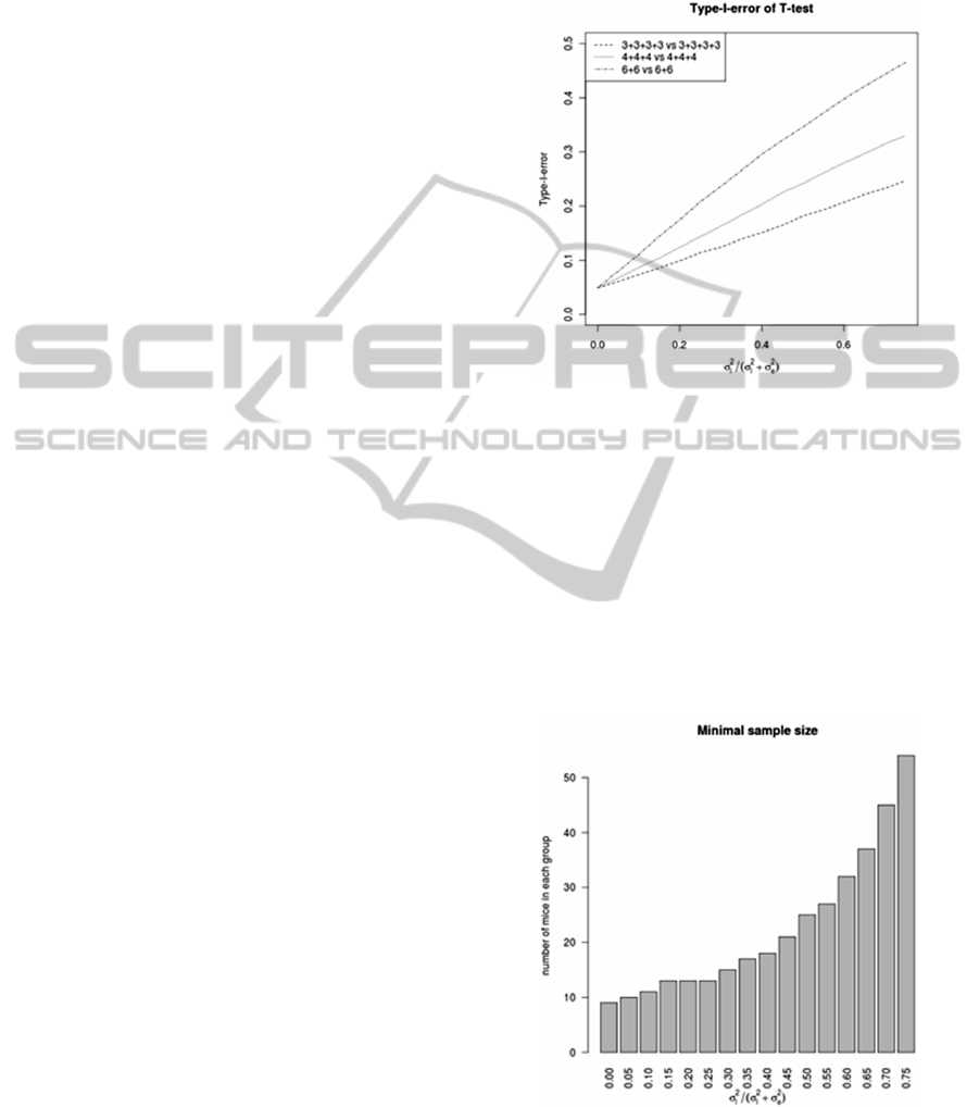
2.3 Simulation Study
We performed a simulation study to quantify the
influence of LE to type-I-error (proportion of false
positives) of T-test (on 5% level). Three scenarios
were considered, each considering 12 mice per
group:
a) Four litters per group, 3 mice per litter
(3+3+3+3 vs. 3+3+3+3)
b) Three litters per group, 4 mice per litter
(4+4+4 vs. 4+4+4)
c) Two litters per group, 6 mice per litter (6+6
vs. 6+6).
The results are visualized on Figure 1. In case of
(average) 25% of residual variability attributed to
LE we get 2.3, 2.9 and 4.2 times as many false
positives as expected, respectively.
Figure 1: Type-I-error of T-test in dependence on
percentage of variability attributed to LE.
The second question is how many mice we need
to get a reasonable chance to significant result of the
test in ANOVA model with random litter effect
(described in Section 4.2). We set the parameters as
follows: 4 mice per litter (e.g. 9 mice are divided
into three litters as 4+4+1), 5% type-I-error
(proportion of false positives), 80% power
(proportion of true positives), and difference
between groups equals two within-litter standard
deviations.
Figure 2: Minimal sample size in dependence on
percentage of variability attributed to LE.
The results are visualized on Figure 2. In case of
(average) 25% of residual variability attributed to
LITTER EFFECT IN MOUSE PHENOTYPIC STUDIES
239

LE, 13 mice per group are needed (minimal sample
size for analogical T-test is 6 mice per group).
3 DISCUSSION
In this paper we have demonstrated presence of LE
in several phenotyping studies.
The consequences are particularly important for
large-scale phenotyping studies (such as databases
of gene knockouts) comparing many traits for a high
number of experimental groups where we predict
higher occurrence of false positive results than
expected.
For illustration let us consider a study of 20
chromosome substitution strains (Nadeau, 2000).
Comparing these strains to control parental strain
result on average in 2-4 false positives (if the design
would be as in Section 2.3) while only 1 false
positive is expected on 5% level.
It is fair to admit that at the moment we do not
know what is behind this effect since mice in the
litter share many common characteristics: not only
mother and father, but also exactly the same
condition during prenatal development, the same
cage, the same day to be born etc. Separation of
these factors will be statistically challenging.
Last but not least, the assumption of independent
observations is not violated only by T-test discussed
in this paper but also by many other methods
commonly used in mouse genetics from QTL
mapping (Broman and Sen, 2009) to microarray
gene expression analysis (Gentleman et al., 2005).
4 MATERIALS AND METHODS
4.1 Datasets
The first data source was our lab notebook with
body weights records of sacrificed mice. We have
restricted ourselves to 28 chromosome substitution
strains and time period from January 2005 to
December 2007. Information about 523 mice (both
males and females, sacrificed between 75 and 81
days) was collected.
Our second data source was Mouse Phenome
Database (MPD), http://www.jax.org/phenome, an
open web-based repository of phenotypic data on
commonly used and genetically diverse inbred
strains
of mice and their derivatives. There were
three large datasets where we were able to recover
litter IDs from mouse IDs: Lake1, Svenson2 and
Tordoff3.
Lake1 (MPD accession number: 199) was a
multi-system analysis of mouse physiology of
C57BL/6J-Chr#
A
/NaJ chromosome substitution
strain panel collected by Jeffrey Lake, Leah Rae
Donahue and Muriel T Davisson. The purpose was
to examine the phenotypic outcome of chromosome
substitution for multiple parameters such as
hematology, blood chemistry, lung function, blood
pressure and pulse, and electrocardiogram. This
survey contains 374 mice from 23 strains.
Svenson2 (Gregorová et al., 2008, MPD
accession number: 219) was an analogical multi-
system physiological survey of mouse physiology in
chromosome substitution strain panel. However, it
was devoted to C57BL/6J-Chr#
PWD
consomics. The
survey contains 399 mice from 18 strains.
Tordoff3 (Tordoff et al., 2007; MPD accession
number: 103) was a survey of calcium and sodium
intake, blood pH and calcium level, and bone and
body composition data in 40 inbred mouse strains to
gain insight into how food and beverage
consumption contribute to diseases such as obesity,
hypertension and diabetes. This survey contains 790
mice.
4.2 Statistical Analysis
The response variable (quantitative trait) 

of an
animal  in an experimental group () and
a litter () was modeled by ANOVA model with
a random litter effect as follows


=

(

)
+

(

)
+

,
(1)
where 
•
is a group fixed effect, 
•
~(0, 


) is a
random litter effect and 
•
~(0, 


) is a random
noise, e.g. Gaussian independent, identically
distributed random variables with zero means and
constant variance.
Residual variability explained by LE (or
attributed to LE) is defined as follows



/(


+


)
(2)
Standard error (SE) of residual variability
explained by LE can be approximated from 


and



by delta method. The distribution of this fraction
is far from bell shape and the calculated SE should
be used as (only) approximation of true value.
Testing for a difference between group means is
a standard test for presence of fixed effect in mixed-
effect model as discussed e.g. in (Verbeke and
Molenberghs, 2000, p. 55). Testing for random litter
BIOINFORMATICS 2011 - International Conference on Bioinformatics Models, Methods and Algorithms
240

effect is a bit more challenging. Two approaches
were implemented:
 Likelihood ratio test as discussed in
(Verbeke and Molenberghs, 2000, p. 65): the
test statistic is a difference in log-likelihood
between models with and without random
effect multiplied by two. Under the null
hypothesis (


=0) it is asymptotically
distributed as a mixture (weights ½ and ½)
of chi-squared distribution with 1 degree of
freedom and constant 0.
 Permutation test: 1000 permutations of
observations within each experimental group
are performed to see how much
exceptionally high is the test statistic (the
observed residual variability explained by
LE). P-value is a fraction of randomly
generated test statistics greater than actually
observed test statistic.
All calculations were done in R 2.9.2, nlme
package was used for LE inference in mixed models.
4.3 Simulation Study
In the first scenario a random sample of 100 000
cases was generated for each considered value of



/(


+


) (from 0.00 to 0.75 by 0.05). For each
case two random vectors were generated such that
observation i of litter l(i) was computed as follows


=
()
+

,
(3)
where 
()
and 

were sampled from distributions
N(0, 


) and N(0, 


), respectively.
For each case T-test was performed and resulting
p-value recorded. The percentage of cases with p-
value below 5% was reported as Type-I-error.
In the second scenario for the same set of
considered values of 


/(


+


) and a temporary
suggestion for possible minimal sample size n we
generated 10 000 samples of two vectors of length n
such that observation i of litter l(i) was computed as
follows


=

(

)
+

+ 2

,
(4)
where  equals zero for the first vector and one for
the second vector; 
()
and 

were sampled from
distributions N(0, 


) and N(0, 


), respectively.
For each case we compared means of vectors by
ANOVA with a random litter effect and record the
p-value. If the percentage of cases with p-value
below 5% was lower than 80% then n was increased
by 1 and the whole procedure was repeated.
ACKNOWLEDGEMENTS
This work was supported in part by the Praemium
Academiae, Academy of Sciences of the Czech
Republic, and by grants IM6837805002 and
AV0Z50520514 from the Ministry of Education,
Youth and Sports of the Czech Republic.
REFERENCES
Broman, K. W., Sen, S., 2009. A Guide to QTL Mapping
with R/qtl. Berlin. Springer.
Gentleman, R., Carey, V., Huber, W., Irizarry, R., Dudoit,
S., 2005. Bioinformatics and Computational Biology
Solutions Using R and Bioconductor. Berlin. Springer.
Glass, G. V., Peckham, P. D., Sanders, J. R., 1972.
Consequences of Failure to Meet Assumptions
Underlying the Fixed Effects Analyses of Variance
and Covariance. Review of Educational Research, 42
(3) pp. 237–288.
Gregorová, S., Divina, P., Storchova, R., Trachtulec, Z.,
Fotopulosova, V., Svenson, K. L., Donahue, L. R.,
Paigen, B., Forejt, J., 2008. Mouse consomic strains:
exploiting genetic divergence between Mus m.
musculus and Mus m. domesticus subspecies. Genome
Research, 18 (3) pp. 509–515.
Grubb, S. C., Maddatu, T. P., et al., 2009. Mouse phenome
database. Nucleic Acids Res, 35 pp. D643–D649.
Haseman, J. K., Kupper L. L., 1979. Analysis of
dichotomous response data from certain toxicological
experiments. Biometrics, 35 (1) pp. 281–293.
Nadeau, J., Singer, J., Matin, A., Lander, E., 2000.
Analysing complex genetic traits with chromosome
substitution strains. Nat. Genet., 24 pp. 221–225.
Silver, L. M., 1995. Mouse Genetics: Concepts and
Applications. Oxford. Oxford University Press.
Tordoff, M. G., Bachmanov, A. A., Reed, D. R., 2000.
Forty mouse strain survey of voluntary calcium intake,
blood calcium, and bone mineral content. Physiol
Behav., 91 (5) pp. 632–643.
Verbeke, G., Molenberghs, G., 2000. Linear Mixed
Models for Longitudinal Data. Berlin. Springer.
LITTER EFFECT IN MOUSE PHENOTYPIC STUDIES
241

Table 1: Litter effect and its statistical significance in three MPD surveys (first part): dataset, variable name and description
(in MPD notation), residual variability (%) explained by LE as defined in (2), its standard error (SE) and p-value of a test
for a submodel without LE (likelihood-ratio and permutation tests).
Dataset Variable Description % explained SE (approx.) p-value (LR test) p-value(perm. test)
Lake1 WBC ## 19901 .... WBC .... total white blood cell (WBC, leukocyte) count (units 17% 9% 0.018 0.003
Lake1 RBC ## 19902 .... RBC .... total red blood cell (RBC, erythrocyte) count (units p
e
27% 9% 0.000 < 0.001
Lake1 mHGB ## 19910 .... mHGB .... measured hemoglobin (HGB) .... g/dL 1% 6% 0.404 0.454
Lake1 HCT ## 19912 .... HCT .... hematocrit (HCT) .... % 26% 8% 0.000 0.002
Lake1 MCV ## 19913 .... MCV .... mean RBC corpuscular vol ume (MCV ) .... fL 33% 8% 0.000 < 0.001
Lake1 MCH ## 19914 .... MCH .... mean RBC corpuscular hemoglobin content (MCH) ..
.
22% 8% 0.001 < 0.001
Lake1 MCHC ## 19915 .... MCHC .... mean RBC corpuscular hemoglobin concentration ( 27% 8% 0.000 < 0.001
Lake1 CHCM ## 19916 .... CHCM .... RBC corpuscular hemoglobin concentration mean (
C
67% 6% 0.000 < 0.001
Lake1 RDW ## 19917 .... RDW .... RBC corpuscular distribution width .... % 60% 7% 0.000 < 0.001
Lake1 HDW ## 19918 .... HDW .... hemoglobin concentration distributi on width (HDW 74% 5% 0.000 < 0.001
Lake1 NEUT ## 19980 .... NEUT .... neutrophils (NEUT) count (units per volume x 103) . 16% 7% 0.003 0.019
Lake1 LYM ## 19981 .... LYM .... lymphocytes (LYMP) count (units per volume x 103) .
.
17% 9% 0.017 0.002
Lake1 MONO ## 19982 .... MONO .... monocytes (MONO) count (units per vol ume x 10
3
39% 8% 0.000 < 0.001
Lake1 EOS ## 19983 .... EOS .... eosinophils (EOS) count (units per volume x 103) ....
n
22% 9% 0.001 0.004
Lake1 LUC ## 19984 .... LUC .... large unstai ned cells (LUC) count (units per volume x 56% 7% 0.000 < 0.001
Lake1 BASO ## 19985 .... BASO .... basophils (BASO) count (units per volume x 103) .... 44% 8% 0.000 < 0.001
Lake1 reticulocytes ## 21917 .... Retic .... reticulocytes (Retic) count (uni ts per volume x 109) 51% 8% 0.000 0.001
Lake1 pct_NEUT ## 19903 .... pct_NEUT .... percent neutrophils (% of total WBC) .... % 15% 7% 0.003 0.025
Lake1 pct_LYM ## 19904 .... pct_LYM .... percent l ymphocytes (% of total WBC) .... % 16% 7% 0.001 0.008
Lake1 pct_MONO ## 19905 .... pct_MONO .... percent monocytes (% of total WBC) .... % 40% 8% 0.000 < 0.001
Lake1 pct_EOS ## 19906 .... pct_EOS .... percent eosinophi ls (% of total WBC) .... % 31% 9% 0.000 0.001
Lake1 pct_LUC ## 19907 .... pct_LUC .... percent l arge unstained cells (% of total WBC) .... 56% 7% 0.000 < 0.001
Lake1 pct_BASO ## 19908 .... pct_BASO .... perce nt basophils (% of total WBC) .... % 45% 8% 0.000 < 0.001
Lake1 pct_Retic ## 19986 .... pct_Retic .... percent reticulocytes (% of total RBC) .... % 49% 8% 0.000 < 0.001
Lake1 cHGB ## 19911 .... cHGB .... cal cul ated hemoglobin (HGB) .... g/dL 39% 8% 0.000 < 0.001
Lake1 PLT ## 19919 .... PLT .... platelet (PLT) count (units per volume x 103) .... n/?L 30% 8% 0.000 < 0.001
Lake1 MPV ## 19920 .... MPV .... mean platelet volume .... fL 56% 8% 0.000 0.003
Lake1 AST ## 19929 .... AST .... aspartate aminotransferase (plasma AST) .... mg/dL 0% 0% 1.000 1.000
Lake1 CHOL ## 19925 .... CHOL .... total cholesterol (pl asma CHOL) .... mg/dL 21% 8% 0.001 < 0.001
Lake1 GLU ## 19927 .... GLU .... glucose (plasma GLU, 4h fast) .... mg/dL 26% 9% 0.000 < 0.001
Lake1 HDL ## 19926 .... HDL .... high density lipoprotein cholesterol (plasma HDL) .... 29% 9% 0.000 < 0.001
Lake1 TFA ## 19930 .... TFA .... total fatty aci ds (plasma TFA) .... mg/dL 47% 8% 0.000 < 0.001
Lake1 TBIL ## 19931 .... TBIL .... total bilirubin (plasma TBIL) .... mg/dL 0% 0% 1.000 1.000
Lake1 TG ## 19928 .... TG .... triglycerides (plasma TG) .... mg/dL 16% 7% 0.004 0.002
Lake1 QRS ## 19941 .... QRS .... interval between beginning and end of QRS comple
x
0% 0% 1.000 1.000
Lake1 PR ## 19942 .... PR .... interval between peak of P-wave to R-wave (PR) .... m 7% 7% 0.145 0.286
Lake1 PQ ## 19943 .... PQ .... interval between peak of P-wave to Q-wave (PQ) ....
m
9% 7% 0.088 0.189
Lake1 QT ## 19944 .... QT .... interval between peak of Q-wave to end of T-wave (
Q
0% 0% 1.000 1.000
Lake1 QTc ## 19945 .... QTc .... rate-corrected QT .... ms 2% 7% 0.374 0.093
Lake1 QT_Dis ## 19946 .... QT_Dis .... QT interval in a string of signals .... ms 15% 7% 0.004 0.036
Lake1 QTc_Dis ## 19947 .... QTc_Dis .... rate corrected QT dispersion .... ms 14% 7% 0.007 0.101
Lake1 HRV ## 19949 .... HRV .... heart rate variabili ty, beats per minute .... n/min 0% 0% 1.000 1.000
Lake1 HR_cv ## 19950 .... HR_cv .... heart rate coeffi cient of variance .... percent 0% 0% 1.000 1.000
Lake1 bp ## 19953 .... bp .... systolic blood pressure .... mmHg 35% 9% 0.000 < 0.001
Lake1 bp_sd ## 19954 .... bp_sd .... systolic blood pressure variability across tests ....
m
15% 8% 0.015 0.006
Lake1 pulse ## 19951 .... pulse .... pulse rate (beats per mi nute) .... n/min 57% 7% 0.000 < 0.001
Lake1 pulse_sd ## 19952 .... pulse_sd .... pul se rate variability across tests (beats per min 23% 8% 0.000 < 0.001
Lake1 BF_roomair breath frequency response, room air 40% 9% 0.000 < 0.001
Lake1 BF_saline breath frequency response, saline 2% 6% 0.399 0.436
Lake1 BF5 breath frequency response to MCh 13% 8% 0.026 0.031
Lake1 BF10 breath frequency response to MCh 19% 8% 0.002 0.002
Lake1 BF20 breath frequency response to MCh 24% 8% 0.000 < 0.001
Lake1 TV_saline ti dal volume response, saline 0% 6% 0.480 0.516
Lake1 TV5 tidal volume response to MCh 19% 8% 0.002 0.018
Lake1 TV10 tidal volume response to MCh 21% 8% 0.000 0.002
Lake1 TV20 tidal volume response to MCh 31% 8% 0.000 < 0.001
Lake1 Penh_roomai
r
Penh response to MCh 25% 9% 0.000 0.003
Lake1 Penh_saline Penh response to MCh 4% 7% 0.294 0.140
Lake1 Penh5 Penh response to MCh 20% 8% 0.001 0.005
Lake1 Penh10 Penh response to MCh 32% 10% 0.000 < 0.001
Lake1 Penh20 Penh response to MCh 29% 9% 0.000 < 0.001
Svenson2 WBC ## 21901 .... WBC .... total white blood cell (WBC, leukocyte) count (units 36% 10% 0.000 < 0.001
Svenson2 RBC ## 21902 .... RBC .... total red blood cell (RBC, erythrocyte) count (uni ts p
e
18% 9% 0.007 0.005
Svenson2 mHGB ## 21909 .... mHGB .... hemoglobin (HGB) .... g/dL 4% 6% 0.211 0.267
Svenson2 HCT ## 21910 .... HCT .... hematocrit (HCT) .... % 31% 9% 0.000 0.005
BIOINFORMATICS 2011 - International Conference on Bioinformatics Models, Methods and Algorithms
242

Table 2: Litter effect and its statistical significance in three MPD surveys (second part): dataset, variable name and
description (in MPD notation), residual variability explained (%) by LE as defined in (2), its standard error (SE) and p-
value of a test for a submodel without LE (likelihood-ratio and permutation tests).
Dataset Variable Description % explained SE (approx.) p-value (LR test) p-value(perm. test)
Svenson2 MCV ## 21911 .... MCV .... mean RBC corpuscular vol ume (MCV ) .... fL 55% 8% 0.000 < 0.001
Svenson2 MCH ## 21912 .... MCH .... mean RBC corpuscular hemoglobin content (MCH) ..
.
0% 0% 1.000 1.000
Svenson2 MCHC ## 21913 .... MCHC .... mean RBC corpuscular hemoglobin concentration ( 5% 6% 0.177 0.334
Svenson2 CHCM ## 21914 .... CHCM .... RBC corpuscular hemoglobin concentration mean (
C
51% 8% 0.000 < 0.001
Svenson2 RDW ## 21915 .... RDW .... RBC corpuscular di stri bution width (RDW) .... % 44% 9% 0.000 < 0.001
Svenson2 HDW ## 21916 .... HDW .... hemoglobin concentration di stributi on width (HDW 57% 8% 0.000 < 0.001
Svenson2 PLT ## 21919 .... PLT .... platelet (PLT) count (units per volume x 103) .... n/?L 5% 7% 0.175 0.116
Svenson2 MPV ## 21920 .... MPV .... mean platelet volume (MPV) .... fL 34% 11% 0.001 0.012
Svenson2 NEUT ## 21921 .... NEUT .... neutrophil (NEUT) count (units pe r vol ume x 103) ... 19% 11% 0.013 0.215
Svenson2 LYM ## 21922 .... LYM .... lymphocyte (LYMP) count (units per volume x 103) ... 35% 10% 0.000 < 0.001
Svenson2 MONO ## 21923 .... MONO .... monocyte (MONO) count (units per volume x 103) 41% 10% 0.000 < 0.001
Svenson2 LUC ## 21926 .... LUC .... large unstai ned cells (LUC) count (units per volume x 22% 8% 0.000 0.003
Svenson2 BASO ## 21925 .... BASO .... basophils (BASO) count (units per volume x 103) .... 44% 9% 0.000 0.004
Svenson2 pctNEUT ## 21903 .... pctNEUT .... percent neutrophils (% of total WBC) .... % 26% 9% 0.000 0.112
Svenson2 pctLYM ## 21904 .... pctLYM .... percent lymphocytes (% of total WBC) .... % 23% 9% 0.000 0.088
Svenson2 pctMONO ## 21905 .... pctMONO .... percent monocytes (% of total WBC) .... % 29% 10% 0.000 < 0.001
Svenson2 pctLUC ## 21907 .... pctLUC .... percent large unstained cel ls (% of total WBC) ....
%
21% 9% 0.001 0.031
Svenson2 pctBASO ## 21908 .... pctBASO .... percent basophils (% of total WBC) .... % 29% 9% 0.000 0.100
Svenson2 pctRetic ## 21992 .... pctRetic .... percent reticulocytes (% of total RBC) .... % 37% 9% 0.000 < 0.001
Svenson2 Retic ## 21917 .... Retic .... reticulocytes (Retic) count (units per volume x 109) 37% 9% 0.000 < 0.001
Svenson2 cHGB ## 21918 .... cHGB .... calculated hemoglobin (HGB) .... g/dL 15% 8% 0.015 0.018
Svenson2 AT3 ## 21941 .... AT3 .... antithrombin III (AT III) anticlotting factor .... % of no
r
30% 9% 0.000 < 0.001
Svenson2 Fib ## 21942 .... Fib .... blood fibrinogen .... mg/dL 20% 9% 0.004 0.024
Svenson2 F8 ## 21943 .... F8 .... clotting factor VIII .... % of normal human value 34% 9% 0.000 < 0.001
Svenson2 TG ## 21962 .... CHOL .... total cholesterol (pl asma CHOL) .... mg/dL 16% 8% 0.011 0.028
Svenson2 HDLD ## 21965 .... HDL .... high density lipoprotein cholesterol (plasma HDL) .... 24% 9% 0.001 < 0.001
Svenson2 AST ## 21967 .... AST .... aspartate aminotransferase (plasma AST, SGOT) .... m 32% 9% 0.000 0.006
Svenson2 FFA ## 21969 .... FFA .... free fatty acids (plasma FFA) .... mEq/L 47% 9% 0.000 < 0.001
Svenson2 TBIL ## 21971 .... TBIL .... total bilirubin (plasma TBIL) .... mg/dL 13% 8% 0.032 0.041
Svenson2 BMD ## 21983 .... BMD .... bone mineral density (BMD) .... g/cm2 20% 10% 0.008 0.003
Svenson2 BMC ## 21984 .... BMC .... bone mineral content (BMC) .... g 37% 9% 0.000 < 0.001
Svenson2 bone_area ??? 33% 9% 0.000 < 0.001
Svenson2 tissue_area ??? 20% 9% 0.002 0.002
Svenson2 RST ??? 3% 8% 0.347 0.110
Svenson2 total_wt ## 21989 .... total_wt .... total body tissue mass .... g 16% 8% 0.017 0.007
Svenson2 fat_wt ## 21991 .... fat_wt .... body fat tissue weight (calculated) .... g 8% 8% 0.120 0.038
Svenson2 lean_wt ## 21990 .... lean_wt .... lean body tissue mass .... g 20% 10% 0.005 0.008
Svenson2 pct_fat ## 21988 .... pct_fat .... percent of tissue mass that i s fat .... % 14% 9% 0.024 0.008
Tordoff3 bw_start ## 10305 .... bw_start .... body wei ght at start of testi ng .... g 32% 7% 0.000 < 0.001
Tordoff3 bw_end ## 10306 .... bw_end .... body weight at end of testing .... g 22% 6% 0.000 < 0.001
Tordoff3 bw_chg ## 10307 .... bw_chg .... fold change in body weight .... fold 17% 7% 0.000 0.144
Tordoff3 CaCl2_pref7 ## 10308 .... CaCl2_pref7 .... preference for 7.5mM CaCl2 solution .... % 10% 5% 0.001 0.004
Tordoff3 CaCl2_pref25 ## 10309 .... CaCl2_pref25 .... preference for 25mM CaCl2 solution .... % 5% 4% 0.077 0.082
Tordoff3 CaCl2_pref75 ## 10310 .... CaCl2_pref75 .... preference for 75mM CaCl2 solution .... % 9% 4% 0.001 0.004
Tordoff3 CaLa_pref7 ## 10311 .... CaLa_pref7 .... preference for 7.5mM CaLa solution .... % 4% 3% 0.069 0.092
Tordoff3 CaLa_pref25 ## 10312 .... CaLa_pref25 .... preference for 25mM CaLa solution .... % 6% 4% 0.027 0.049
Tordoff3 CaLa_pref75 ## 10313 .... CaLa_pref75 .... preference for 75mM CaLa solution .... % 2% 3% 0.228 0.229
Tordoff3 NaCl _pref75 ## 10315 .... NaCl_pre f75 .... preference for 75mM NaCl solution .... % 16% 5% 0.000 < 0.001
Tordoff3 NaCl _pref225 ## 10316 .... NaCl_pre f225 .... preference for 225mM NaCl solution .... % 13% 5% 0.000 < 0.001
Tordoff3 NaLa_pref25 ## 10317 .... NaLa_pref25 .... preference for 25mM NaLa sol ution .... % 4% 3% 0.097 0.114
Tordoff3 NaLa_pref75 ## 10318 .... NaLa_pref75 .... preference for 75mM NaLa sol ution .... % 14% 6% 0.000 0.002
Tordoff3 NaLa_pref225 ## 10319 .... NaLa_pref225 .... preference for 225mM NaLa sol ution .... % 15% 6% 0.000 0.001
Tordoff3 bleeding_tim
e
## 10320 .... bleedi ng_ti me .... time from tail cut to 1/2 tube of blood coll 15% 5% 0.000 0.111
Tordoff3 ionized_Ca ## 10321 .... ionized_Ca .... blood ionized calcium .... mg/dL 36% 6% 0.000 < 0.001
Tordoff3 pH ## 10322 .... pH .... blood pH .... pH 28% 6% 0.000 < 0.001
Tordoff3 adj_ionized_
C
## 10323 .... adj_ionized_Ca .... blood ionized calcium adjusted to pH 7.4 . 39% 6% 0.000 < 0.001
Tordoff3 total_calci um ## 10324 .... total_calcium .... pl asma total calcium .... mg/dL 21% 5% 0.000 < 0.001
Tordoff3 BMD ## 10326 .... BMD .... bone mineral density .... g/cm2 29% 6% 0.000 < 0.001
Tordoff3 BMC ## 10327 .... BMC .... bone mineral content .... g 21% 6% 0.000 < 0.001
Tordoff3 lean_wt ## 10328 .... lean_wt .... calculated weight of lean tissue .... g 44% 6% 0.000 < 0.001
Tordoff3 fat_wt ## 10329 .... fat_wt .... calculated weight of fat ti ssue .... g 30% 6% 0.000 < 0.001
Tordoff3 total_wt ## 10330 .... total_wt .... total weight (lean + fat) .... g 44% 6% 0.000 < 0.001
Tordoff3 pct_fat ## 10331 .... pct_fat .... percent fat .... % 13% 5% 0.000 < 0.001
Tordoff3 pct_lean ## 10332 .... pct_lean .... percent l ean .... % 13% 5% 0.000 < 0.001
LITTER EFFECT IN MOUSE PHENOTYPIC STUDIES
243