TOWARDS ROUTING FOR AUTONOMOUS ROBOTS

Using Constraint Programming in an Anytime Path Planner

Roman Barták

Faculty of Mathematics and Physics, Charles University, Praha, Czech Republic

Michal Zerola

Faculty of Nuclear Sciences and Physical Engineering, Czech Technical University, Praha, Czech Republic

Stanislav Slušný

Institute of Computer Science, Academy of Sciences of the Czech Republic, Praha, Czech Republic

Keywords: Vehicle routing, Autonomous robots, Constraint programming, Optimisation.

Abstract: Path planning is one of the critical tasks for autonomous robots. In this paper we study the problem of

finding the shortest path for a robot collecting waste spread over the area such that the robot has a limited

capacity and hence during the route it must periodically visit depots/collectors to empty the collected waste.

This is a variant of often overlooked vehicle routing problem with satellite facilities. We present two

approaches for this optimisation problem both based on Constraint Programming techniques. The former

one is inspired by the operations research model, namely by the network flows, while the second one is

driven by the concept of finite state automaton. The experimental comparison and enhancements of both

models are discussed with emphasis on the further adaptation to the real world environment.

1 INTRODUCTION

Recent advances in robotics have allowed robots to

operate in cluttered and complex spaces. However,

to efficiently handle the full complexity of the real-

world tasks, new deliberative planning strategies are

required. In this paper, we deal with the robot

performing a routine task of collecting waste for

example in large department stores where the remote

control is boring for humans and hence error prone.

In particular, we solve the problem of planning a

route for a single robot such that all waste is

collected, robot’s capacity is never exceeded, and

the route is as short as possible. We assume the

environment to be known and not changing, in

particular, the location of waste and depots is known

and the robot knows how to move between these

locations. To handle changes in the environment we

focus on anytime planning algorithms that can be re-

run when the initial task changes, for example, the

distances between the navigation points change due

to cluttered areas. We propose to use Constraint

Programming (CP) to solve the problem because of

the flexibility of CP. This allows us to use a base

model describing the core task and to add new

constraints later when necessary. Such a new

constraint could be the restriction on allowed

combinations of entrance and exit routes when

collecting the waste or visiting the depot for robots

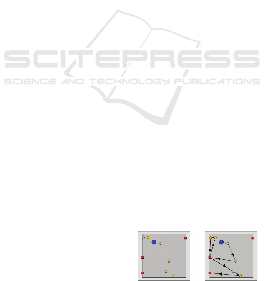
with limited manoeuvring capabilities. Figure 1

gives an example of the initial environment (left)

and the found path for the robot (right).

Figure 1: Example of 6+3 robot planning task. The robot

(the big circle) collects waste (six small circles) and uses

collectors (three squares) to empty the bin when it is full.

313

Barták R., Zerola M. and Slušný S..

TOWARDS ROUTING FOR AUTONOMOUS ROBOTS - Using Constraint Programming in an Anytime Path Planner.

DOI: 10.5220/0003178703130320

In Proceedings of the 3rd International Conference on Agents and Artiﬁcial Intelligence (ICAART-2011), pages 313-320

ISBN: 978-989-8425-40-9

 2011 SCITEPRESS (Science and Technology Publications, Lda.)

The task we are dealing with is to develop a

robot solving a specific routing problem – an often

overlooked variant of the standard Vehicle Routing

Problem (VRP). In our setting, the robot has to clean

out a collection of waste spread in a building, but

under the condition of not exceeding its internal

storage capacity at any time. The storage tank can be

emptied in one of available collectors. The goal is to

come up with the routing plan minimising the

travelled trajectory. This is a similar setting to a

Vehicle Routing Problem with Satellite Facilities

(VRPSF) studied in (Bard et al., 1998), where the

task is to deliver goods rather than to collect waste.

Our primary goal is to develop an algorithm that

returns good solutions in a short time (almost

anytime algorithm) and that can be easily extended

by additional constraints. Hence ad-hoc exact

techniques are not appropriate due to long runtime

and limited extendibility and we decided to use

Constraint Programming (CP) to solve the problem.

Neither of existing CP-oriented works solves the

above problem, but we can use them as the initial

motivation for the design of our constraint model.

Most of the routing models are based on the

formulation of the problem using network flows

(Simonis, 2006) so we also proposed a constraint

model based on this standard technique.

Nevertheless, the performance of this model was not

satisfactory in our experiments so we proposed a

radically new approach to model the problem using

a finite state automaton. In our preliminary

experiments, this model outperforms the traditional

model and can solve larger instances of the problem.

The paper is organised as follows. We will first

formally describe the problem to be solved. Then we

will formulate the traditional model based on

network flows that we customised to solve our

problem. After that we will describe the novel model

based on finite state automata. The paper will be

concluded by the preliminary experimental results.

2 PROBLEM FORMULATION

Recall that we are solving a single robot path

planning problem with the capacity constraint. The

robot’s environment consists of the navigation

points defined by the locations of waste and

collectors. We use a mixed weighted graph (V, E)

with both directed and undirected edges to represent

this environment. The reason for using undirected

edges is minimising the size of the representation.

The set of vertices V = {I}  W  C  {D} consists

of the initial position I, the set W of waste vertices,

the set C of collectors and the destination vertex D.

From the initial position the robot has to visit some

waste so we have directed arcs from I to all vertices

in W. The robot can travel between the waste

vertices so we assume a complete undirected graph

between vertices in W. From any waste vertex the

robot can go to a collector so we use a directed edge

there and from any collector we can go to any waste

which is again modelled using a directed edge. We

need directed edges here as we need to count the

number of incoming and ongoing edges for the

collectors. There are no edges between the collector

vertices. As mentioned, we use a dummy destination

vertex that is connected to all collector vertices by a

directed edge. The weight of each edge describes the

distance between the navigation points. The edges

going to the dummy destination vertex D has zero

weight so the robot can actually finish at any

collector. The task to find a minimal-cost path

starting at I, finishing at D and visiting each vertex

in W exactly once such that the number of any

consecutive vertices from W does not exceed the

given capacity of the robot. Figure 2 shows the

schema of the graph with the navigation points.

Figure 2: A schema of the graph describing the robot’s

environment with the navigation points.

3 CP MODEL BASED ON

NETWORK FLOWS

The first model that we propose resembles the

traditional operations research models of vehicle

routing problems based on network flows and

Kirchhoff’s laws. Basically, we are describing

whether or not the robot traverses a given edge. For

every edge e we introduce a binary decision variable

stating whether the edge is used in the path (value

1) or not (value 0).

Let IN(v) and OUT(v) denote the set of incoming

and outgoing directed edges for the vertex v. For

example, for v  W the set IN(v) contains the arc

from the vertex I and the arcs from the vertices in C.

Let ICD(v) be a set of undirected edges incident to

vertex v. This set is empty for the collector vertices;

for waste vertices it contains undirected edges

connecting the vertex with other waste vertices. The

following constraints describe that the robot leaves

the initial position I, reaches the destination position

ICAART 2011 - 3rd International Conference on Agents and Artificial Intelligence

314

D, and enters each collector c the same number of

times as it leaves it:



eOUT(I)

= 1, 

eIN(D)

= 1,

(1)

c  C: 

eOUT

(

)

= 

eIN

(

)

(2)

Let us now describe the constraint that each waste

vertex w is visited exactly once. It means that

exactly two edges incident to a waste vertex w are

active (used in the solution path) and there can be at

most one active incoming and outgoing directed

edge connecting the waste with the collectors or

with the initial node.

w  W: 

eOUT

(

)

 IN

(

)

 ICD

(

)

= 2 ,

(3)

w  W: 

eOUT

(

)

 1,

(4)

w  W: 

eIN

(

)

 1,

(5)

The above constraints describe any path leading

from I to D, but they also allow isolated loops as

Figure 3 shows. This is a known issue of this type of

model that is usually resolved by additional sub-tour

elimination constraints forcing any two subsets of

vertices to be connected.

Figure 3: An ineligible loop (left) satisfying the routing

(Kirchhoff’s) constraints.

In our particular setting, we need to carefully

select these pairs of subsets of vertices because there

could be collector vertices that are not visited.

Hence, we consider any pair of disjoint subsets

, S

 (W  C), such that neither S

nor S

consists of collector vertices only. More precisely,

we assume the pairs of subsets S

, S

such that:

= (W  C) \ S

, S

 W  , S

 W  

(6)

The sub-tour elimination constraint can then be

expressed using the following formula ensuring that

there is at least one active edge between S

and S



eE: e  S

   e  S

 

 1.

(7)

Clearly, there is an exponential number of such pairs

and S

, which makes it impractical to introduce

all such sub-tour elimination constraints. Some

authors (Pop, 2007) propose using single or multi-

commodity flow principles to reduce the number of

constraints by introducing auxiliary variables.

However, our combination of directed and

undirected edges makes it complicated to use this

approach so we rather applied another approach

based on lazy (on-demand) insertion of sub-tour

elimination constraints. Briefly speaking, we start

with the model without the sub-tour elimination

constraints and we find a solution. If the solution

forms a valid path then we are done. Otherwise we

identify the isolated loops, add the sub-tour

elimination constraints for them and start the solver

with the updated model. This process is repeated

until a valid path is found. Obviously, it is a

complete procedure because in the worst case, all

sub-tour elimination constraints are added.

It remains to define the constraints describing the

limited capacity of the robot. For this purpose we

introduce auxiliary non-decision capacity variables

for every waste vertex v  W. These variables

indicate the amount of waste in the robot after

visiting the particular vertex. The non-decision

character of the variables means that they are not

instantiated by the search procedure, but they are

instantiated by the inference procedure only. In

particular, if their domain becomes empty during

inference then it indicates inconsistency. The

following constraints are used during the inference

(w  W). First, if the waste vertex w is visited

directly after the collector then there is exactly one

waste in the robot:



eIN(w)

= 1  C

= 1

(8)

Second, if the waste vertices u and v are visited

directly before respectively after w (or vice versa)

then the following constraints must hold between the

capacity variables:



e,f



ICD(w), e = {u,w}, f = {w,v}:

+ X

= 2  | C

– C

| = 2

(9)



e = {u,w}



ICD(w):

–

= 1

(10)

Finally, to restrict the capacity of the robot by

constant cap we use the following constraints for the

capacity variables:

w  W: 1  C

 cap.

(11)

The objective function to be minimised is the total

cost of edges used in the solution path:

Obj = 

eE

. weight(e),

(12)

where weight(e) is the weight of edge e.

TOWARDS ROUTING FOR AUTONOMOUS ROBOTS - Using Constraint Programming in an Anytime Path Planner

315

3.1 Search Procedure

The constraint model describes how the inference is

performed so the model needs to be accompanied by

the search procedure that explores the possible

instantiations of variables X

Our search strategy resembles the greedy

approach for solving Travelling Salesman Problems

(TSP) (Ausiello et al., 1999). The variable X

for

instantiation is selected in the following way. If the

path is empty, we start at the initial position I and

instantiate the variable X

{I,w}

such that weight({I,w})

is the smallest among the weights of arcs going from

I. By instantiating the variable we mean setting it to

1; the alternative branch is setting the variable to 0.

If the path is non-empty then we try to extend it to

the nearest waste. Formally, if u is the last node in

the path then we select the variable X

{u,w}

with the

smallest weight({u,w}), where w is a waste vertex. If

this is not possible (due to the capacity constraint),

we go to the closest collector.

The optimisation is realised by the branch-and-

bound approach: after finding a solution with the

total cost Bound, the constraint Obj < Bound is

posted and search continues until any solution is

found. The last found solution is the optimum.

4 CP MODEL BASED ON

FINITE STATE AUTOMATA

The second model that we propose brings a radically

new approach not seen so far when modelling VRPs

or TSPs. Recall that we are looking for a path in the

graph that satisfies some additional constraints. We

can see this path as the word in a certain regular

language. Hence, we can base the model on the

existing regular constraint (Pesant, 2004). This

constraint allows a more global view of the problem

so the hope is that it can infer more information than

the previous model and hence decreases the search

space to be explored.

First, it is important to realise that the exact path

length is unknown in advance. Each waste vertex is

visited exactly once, but the collector vertices can be

visited more times and it is not clear in advance how

many times. Nevertheless, it is possible to compute

the upper bound on the path’s length. Let us assume

that the path length is measured as the number of

visited vertices, the robot starts at the initial position

and finishes at some collector vertex (we will use the

dummy destination in a slightly different meaning

here), and the weight/cost of arcs is non-negative.

Let K = |W| be the number of waste vertices and

cap  1 be the robot’s capacity. Then the maximal

path length is 2K+1. This corresponds to visiting a

collector vertex immediately after visiting a waste

vertex. Recall that each waste vertex must be visited

exactly once and there is no arc between the

collector vertices.

Our model is based on four types of constraints.

First, there is a restriction on the existence of a

connection between two vertices – a routing

constraint. This constraint describes the routing

network (see Figure 2). It roughly corresponds to the

constraints (1)-(5) from the previous model. Note

that the sub-tour elimination constraints (6)-(7) are

not necessary here. Second, there is a restriction on

the robot’s capacity stating that there in no

continuous subsequence of waste vertices whose

length exceeds the given capacity – a capacity

constraint. This constraint corresponds to the

constraints (8)-(11) from the previous model. Third,

each waste must be visited exactly once, while the

collectors can be visited more times (even zero

times) – an occurrence constraint. This restriction

was included in the constraints (1)-(5) of the

previous model, while we model it as a separate

constraint. Finally, each arc is annotated by a weight

and there is a constraint that the sum of the weights

of used arcs does not exceed some limit – a cost

constraint. This constraint is used to define the total

cost of the solution as in (12).

In the constraint model we use three types of

variables. Let N = 2K + 1 be the maximal path

length. Then we have N variables Node

, N variables

Cap

, and N variables Cost

(i = 1,...,N) so we

assume the path of maximal length. Clearly, the real

path may be shorter so we introduce a dummy

destination vertex that fills the rest of the path till the

length N. In other words, when we reach the dummy

vertex, it is not possible to leave it. This way, we can

always look for the path of length N and the model

gives flexibility to explore the shorter paths too.

The semantic of the variables is as follows. The

variables Node

describe the path hence their domain

is the set of numerical identifications of the vertices.

We use positive integers 1,...,K (K = |W|) to identify

the waste vertices, K+1,...,K+L for the collector

vertices (L = |C|), and 0 for the dummy destination

vertex. In summary, the initial domain of each

variable Node

consists of values 0,..., K+L. Cap

the used capacity of the robot after leaving vertex

Node

(Cap

= 0 as the robot starts empty), the initial

domain is {0,…, cap}. Cost

is the cost of the arc

used to leave the vertex Node

(Cost

= 0), the initial

domain consists of non-negative numbers. Formally:

ICAART 2011 - 3rd International Conference on Agents and Artificial Intelligence

316

i = 1,…,N (N = 2K + 1):

0  Node

 K+L

0  Cap

 cap, Cap

= 0

0  Cost

, Cost

= 0

(13)

We will start the description of the constraints with

the occurrence constraint saying that each waste

vertex is visited exactly once. This can be modelled

using the global cardinality constraint (Régin, 1996)

over the set {Node

,…, Node

}. The constraint is set

such that the each value from the set {1,.., K} is

assigned to exactly one variable from {Node

,…,

Node

} – each waste node is visited exactly ones.

The values {0, K+1,…, K+L} can be used any

number of times. Formally:

gcc({Node

,…, Node

{v:[1,1] v = 1,…,K,

0:[0,],

v:[0,] v = K+1,…,K+L}

(14)

where v:[min,max] means that value v is assigned to

at least min and at most max variables from

{Node

,…, Node

The gcc constraint allows specifying the number

of appearances of the value using another variable

rather than using a fixed interval as in (14). Let D be

the variable describing the number of appearances of

value 0 (identification of the dummy vertex) in the

set {Node

,…, Node

}, then we can use the

following constraints instead of (14):

gcc({Node

,…, Node

{v:[1,1] v=1,…,K,

0:D,

v:[0,] v=K+1,…,K+L})

Node

N-D

> 0

(15)

(16)

The constraint (16) says that Node

N-D

is not a

dummy vertex; actually it is the last real vertex in

the path. We can also set the upper bound for D by

using the information about the minimal path length

(MinPathLength is a constant computed in advance):

D  N – MinPathLength

(17)

These additional constraints (16) and (17) are not

necessary for the problem specification but they

improve inference (we use them in experiments).

The cost constraint can be easily described as

Obj = 

i=1,…,N

Cost

(18)

so we can use the constraints Obj < Bound in the

branch-and-bound procedure exactly the same way

as in the previous model.

For the cost constraint to work properly we need

to set the value of Cost

variables. Recall that Cost

the cost/weight of the arc going from vertex Node

vertex Node

i+1

. Hence, we can connect the Cost

variables with the Node variables when specifying

the routing constraint. In particular, we use the

ternary constraints over the variables Node

, Cost

Node

i+1

i=1,…N-1. This set of constraints

corresponds to the idea of slide constraint (Bessiere

et al., 2007). We implement the constraint between

the variables Node

, Cost

, Node

i+1

as a ternary

tabular (extensionally defined) constraint; let us call

it link, where the triple (p, q, r) satisfies the

constraint if there is an arc from the vertex p to the

vertex r with the cost q. In other words, this table

describes the original routing network with the costs

extended by the dummy vertex. Formally:

link(p,q,r)  eE: e = (p,r), q = weight(e)

(19)

 (q = r = 0



(p = 0  p > K)



i = 1,…,2K: link(Node

, Cost

, Node

i+1

)

(20)

It remains to show how the capacity constraint is

realised. Briefly speaking, we use a similar approach

as for the routing constraint. The capacity constraint

is realised using a set of ternary constraints over the

variables Cap

, Node

i+1

, Cap

i+1

i=1,…N-1, again

exploiting the idea of slide constraint. The constraint

is implemented using a tabular constraint, let us call

it capa, with the following semantics. Triple (p, q, r)

satisfies this constraint if and only if

 q is an identification of a collector vertex (q > K)

or a dummy vertex (q = 0) and r = 0

 q is an identification of a waste node (0 < q  K)

and r = p+1.

Recall that the domain of capacity variables is

{0,…,cap} so we never exceed the capacity of the

robot. Formally:

capa(p,q,r)  q = r = 0

(21)

 (q > K



r = 0)

 (0 < q





r = p+1)



i = 1,…,2K: capa(Cap

, Node

i+1

, Cap

i+1

)

(22)

Any solution to the above described constraint

satisfaction problem defines a valid solution of our

single robot path planning problem with the capacity

constraint. Vice versa, any solution to the path

planning problem is also a feasible solution of the

specified constraint satisfaction problem. We omit

the formal proof due to limited space.

4.1 Search Procedure

Similarly to the previous model, it is important to

specify the search strategy. In this second model,

TOWARDS ROUTING FOR AUTONOMOUS ROBOTS - Using Constraint Programming in an Anytime Path Planner

317

only the variables Node

are the decision variables –

they define the search space. It is easy to realise that

the inference through the routing constraints (20)

decides the values of the Cost

variables and the

inference through the capacity constraints (22)

decides the values of the Cap

variables provided

that the values of all variables Node

are known.

When searching for the solution we first use a

greedy approach to find the initial solution (the

initial cost). This greedy algorithm instantiates the

variables Node

in the order of increasing i in such a

way that the arc with the smallest cost is preferred.

We select the node to which the least expensive arc

from the previously decided node leads. Naturally,

the capacity constraint is taken into account so only

the nodes such that the capacity is not exceeded are

assumed. This search procedure corresponds to the

search strategy of the previous model. The

difference in models allows us to use a fixed

variable ordering in the model based on finite

automata which simplifies implementation of the

search procedure. This second model also has fewer

decision variables but a larger branching factor.

To find the optimal solution we use a standard

branch-and-bound approach with restarts. To

instantiate the Node variables we use the min-dom

heuristic for the variable selection, that is, the

variable with the smallest current domain is

instantiated first. We select the values in the order

defined in the problem (the waste nodes are tried

before the collector nodes). Exactly like in the first

model after finding a solution with the total cost

Bound, the constraint Obj < Bound is posted and

search continues until any solution is found. The last

found solution is the optimum. Note that using the

well known and widely applied min-dom heuristic

for the variable selection is meaningful in this model

because we have larger domains, while the same

heuristic is useless for the previous model which

uses binary domains.

5 EXPERIMENTAL RESULTS

In this section we will present the preliminary

experimental evaluation of the presented solving

techniques. As there is no standard benchmark set

for the studied problem, we generated own problem

instances. We used a square-sized robot arena where

the positions of the waste and the initial location of

the robot were uniformly distributed. The collectors

were uniformly distributed along the boundaries of

the arena and the weights set up as a point-to-point

distance using the Euclidean metric. All the

following measurements were performed on Intel

Xeon CPU@2.5GHz with 4 GB of RAM, running a

Debian GNU Linux operating system.

5.1 Performance of the

Network Flow Model

As stated earlier, the model based on network flows

corresponds to the traditional operations research

approach, but we modified the model to describe

specifics of our robot routing problem. The model

was implemented in Java using Choco

(http://choco.emn.fr), an open-source constraint

programming library. The optimisation search

strategy uses the built-in branch-and-bound method,

while all constraints correspond to the mathematic

formulations described earlier.

Figure 4 shows the runtime (a logarithmic scale)

to obtain the optimal solution as a function of the

instance size measured by the number of waste and

by the number of collectors. We generated 15

instances for each problem size and the graph shows

the average time the solver needs for finding and

proving the optimality of the solution. The capacity

of robot was 3.

Figure 4: Runtime (seconds) for the network flow model.

As already mentioned in (Bard et al., 1998), the

satellite facilities in VRP (or collectors in robotics

case) heavily increase the complexity of the

problem. The initial experiment shows that the

runtime increases exponentially with the number of

waste but the runtime is not significantly affected by

the increased number of collectors. In fact it seems

that for different quantities of waste there are

different numbers of collectors where the best

runtime is achieved. This is an interesting

observation claiming that for a given number of

waste there is some number of collectors that gives

1E‐06

1E‐05

0,0001

0,001

0,01

0,1

100

ICAART 2011 - 3rd International Conference on Agents and Artificial Intelligence

318

the best result. Nevertheless, this observation

requires additional experiments to confirm it.

5.2 Performance of the Finite State

Automaton Model

The network flow model represents a standard

approach to solving the Vehicle Routing Problems

so we compared our novel constraint model based

on the finite state automaton directly to this

approach. The second model was implemented in

SICStus Prolog (http://www.sics.se/sicstus). Figure

5 shows the runtime (a logarithmic scale) to obtain

the optimal solution using the constraint model

based on finite state automata using the same

problems as for the model based on network flows

(Figure 4). The result also shows the exponential

grow with the increased number of waste and

weaker dependence on the number of collectors.

Figure 5: Runtime (seconds) for the FSA model.

Figure 6: Time difference (seconds) between the CP

models. Positive values means that the model based on

finite state automata is faster.

To directly compare both models, we generated a

difference graph showing the difference of runtimes

for the network model and for the automata model –

the values above zero mean faster automata model,

while the times below zero mean faster network

model. Figure 6 shows these difference times. The

conclusion drawn from this graph is as follows. The

automata-based model is visibly better for a smaller

number of collectors where the problem is more

constrained and the capacity constraints can prune

more of the search space. A bit surprisingly, it seems

that the network-based model is better when the

number of collectors becomes larger. This feature

will require a further investigation.

6 CONCLUSIONS

We proposed two constraints models for deliberative

planning of the robot picking up all waste in a

known environment and putting them to collectors

while assuming a limited capacity of the robot. We

used a constraint model based on network flows that

is traditionally applied to this type of routing

problems and we developed a completely new model

based on finite state automata. Using the constraint

programming techniques allowed us to naturally

define the underlying model for which the solver

was able to find the first solution in hundreds of

microseconds on problems of reasonable size. The

preliminary experiments showed some interesting

behaviour of the model in relation to the number of

collectors that we shall further investigate.

ACKNOWLEDGEMENTS

The research is supported by the Czech Science

Foundation under the contract P202/10/1188, by

the grants LC07048 and LA09013 of the Ministry of

Education of the Czech Republic, and by the project

KJB100300804 of GA AV ČR.

REFERENCES

Ausiello, G., Crescenzi, P., Kann, V., Marchetti-

Spaccamela, A., Protasi, M., 1999. Complexity and

Approximation: Combinatorial Optimization Problems

and Their Approximability Properties, Springer.

Bard, J. F., Huang, L., Dror, M., Jaillet, P., 1998. A branch

and cut algorithm for the VRP with satellite facilities.

IIE Transactions 30(9), Springer, pp. 821-834.

Bessiere, C., Hebrard, E., Hnich, B., Kiziltan, Z.,

Quimper, C. G., Walsh, T., 2007. Reformulating

global constraints: The Slide and Regular Constraints.

1E‐06

1E‐05

0,0001

0,001

0,01

0,1

100

‐200

‐150

‐100

‐50

100

150

TOWARDS ROUTING FOR AUTONOMOUS ROBOTS - Using Constraint Programming in an Anytime Path Planner

319

In Proceedings of SARA, LNCS 4612, Springer, pp.

80-92.

Pesant, G., 2004. A Regular Language Membership

Constraint for Finite Sequences of Variables. In

Principles and Practice of Constraint Programming,

LNCS 3285, Springer, pp. 482-495.

Pop, P. C., 2007. New Integer Programming Formulations

of the Generalized Travelling Salesman Problems.

American Journal of Applied Sciences 11, pp. 932-

937.

Régin, J. C., 1996. Generalized Arc Consistency for

Global Cardinality Constraint. In Proceedings of

AAAI, AAAI Press, pp. 209-215.

Simonis, H., 2006. Constraint applications in networks. In

Handbook of Constraint Programming, Elsevier, pp.

875-903.

ICAART 2011 - 3rd International Conference on Agents and Artificial Intelligence

320