SURFACE ROUGHNESS MODELLING AND OPTIMIZATION IN
CNC END MILLING USING TAGUCHI DESIGN
AND NEURAL NETWORKS
Menelaos Pappas, John Kechagias, Vassilis Iakovakis
Department of Mechanical Engineering, Technological Educational Institute of Larissa, Larissa 41110, Greece
Stergios Maropoulos
Department of Mechanical Engineering, Technological Educational Institute of Western Macedonia, Kozani 50100, Greece
Keywords: Artificial neural network, Cutting parameters, Process optimization, Surface quality.
Abstract: A Neural Network modelling approach is presented for the prediction of surface texture parameters during
end milling of aluminium alloy 5083. Eighteen carbide end mill cutters were manufactured by a five axis
grinding machine and assigned to mill eighteen pockets having different combinations of geometry
parameters and cutting parameter values, according to the L
18
(2
1
x3
7
) standard orthogonal array. A feed-
forward back-propagation NN was developed using data obtained from experimental work conducted on a
CNC milling machine center according to the principles of Taguchi’s design of experiments method. It was
found that NN approach can be applied easily on designed experiments and predictions can be achieved, fast
and quite accurately.
1 INTRODUCTION
Aluminium 5083 is generally supplied as a flat
rolled product in plate form and it has the highest
strength of the non-heat treatable alloys. Although
there is no specific machinability data the Al 5083 is
machinable by conventional means.
The machinability of an engineering material
denotes its adaptability to machining processes with
regard to factors such as cutting forces, tool wear
and surface roughness. Surface roughness plays an
important role on the product quality and is a
parameter of great importance in the evaluation of
the machining accuracy (Kechagias et al., 2009;
2010).
The surface roughness of parts produced by
material removal processes is affected by various
factors such as material properties, tool geometry,
cutting parameters, etc. Thus parameter design for a
material is useful in order to have the best
performance and consequently decrease the quality
loss of a process (Phadke, 1989).
A number of attempts, which study surface
quality, cutting forces, tool wear, and cheap
morphology, during end milling, are reported in the
literature. Most of these studies refer to specific
cutting conditions, such as the tool-workpiece
material and the cutting tool geometry (Engin and
Altintas, 2001; Yun and Cho 2000).
The current research work studies the influence
of the cutting parameters and the end cutter
geometry parameters during end milling of Al alloy
5083 on the surface texture parameters; arithmetical
mean roughness (R
a
), maximum peak (R
y
), and ten-
point mean roughness (R
z
).
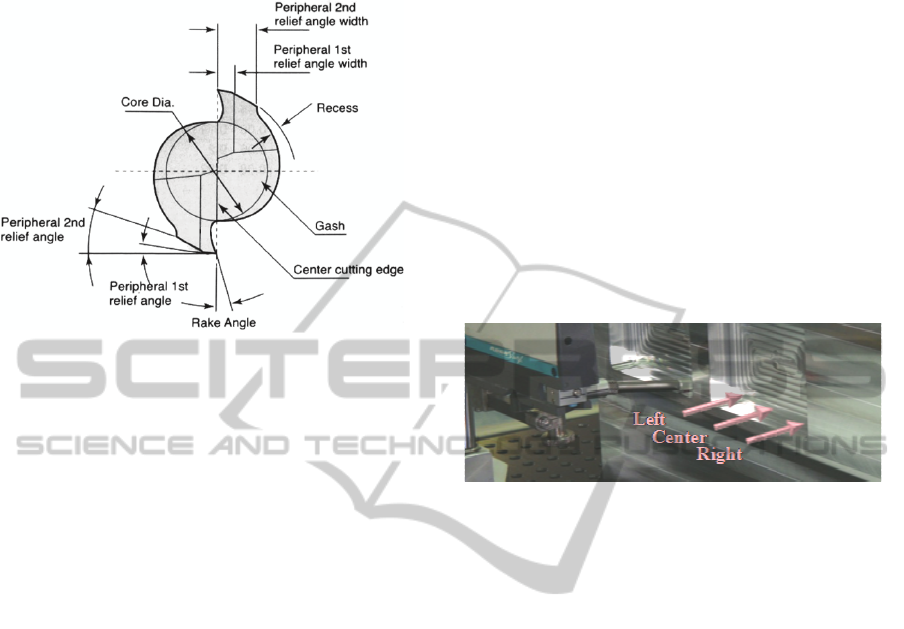
The two-flute end cutter geometry parameters
tested are the core diameter (%), flute angle (
o
), rake
angle (
o
), peripheral 1st relief angle (
o
) and
peripheral 2nd relief angle (
o
). The core diameter is
measured as a percentage of the end mill cutter
diameter. End mill cutter geometry parameters can
be seen in Figure 1.
The above parameters were combined with
cutting depth (mm), cutting speed (rpm) and tool
feed (mm/flute) using an L
18
(2
1
x3
7
) orthogonal
matrix experiment and the results were used to built
a NN model in order to predict/estimate the surface
roughness indicator response according to the
595
Pappas M., Kechagias J., Iakovakis V. and Maropoulos S..
SURFACE ROUGHNESS MODELLING AND OPTIMIZATION IN CNC END MILLING USING TAGUCHI DESIGN AND NEURAL NETWORKS .
DOI: 10.5220/0003180505950598
In Proceedings of the 3rd International Conference on Agents and Artificial Intelligence (ICAART-2011), pages 595-598
ISBN: 978-989-8425-40-9
Copyright
c
 2011 SCITEPRESS (Science and Technology Publications, Lda.)

geometry and cutting parameters of the end milling
process.
Figure 1: Two flute end mill cutter geometry (front view).
NNs have also been effectively used in the past
not only for modelling and optimization of
manufacturing processes but also in case of highly
non-linear non-manufacturing problems
(Chryssolouris et al., 2004; Kechagias and
Iakovakis, 2009; Markopoulos et al., 2006).
2 EXPERIMENT
Aluminum alloy 5083 is a non-heat treatable alloy. It
has very good corrosion resistance; it is easily
welded and is of high strength.
End milling pockets were performed on a
DECKEL MAHO DMU 50V-monoBLOCK 5-axis
universal high speed machining center. The max
power of the machine tool and the max spindle
speed were 18,9 kW and 14.000 r/min respectively.
The two flute carbide end mill cutters were
manufactured using the five axis Hawemat 2001
grinding machine. NAMROTO CAM program was
used to simulate the grinding process in order to
avoid collision among machine components.
Table 2 was designed using the Taguchi
methodology (Phadke, 1989) and corresponds to the
standard L
18
(2
1
x3
7
) orthogonal array. In this
method, the main parameters, which are assumed to
have an influence on the process results, are located
in different rows in a designed orthogonal array and
the results can be analyzed using an analysis of
means and analysis of variance, in a similar way as a
full factorial design, were conducted.
The geometry parameter values of each of the
eighteen two-flute end mill cutters are shown in
columns A to E of Table 2. All of the eighteen
carbide cutters have a diameter of 8 mm. The cutting
parameter values during eighteen pockets are shown
in columns F to H of Table 2, too.
Each of the eighteen end mill cutters cut a pocket
of 100 mm x 64 mm and 15 mm in depth on the two
faces of an Al 5083 plate of 500 mm x 280 mm and
60 mm in depth. The two faces were finished with a
face mill cutter, 50 mm in diameter, and two
recesses were constructed in order to fix the Al plate
on to the machine center chuck. The cutting
parameter values for each pocket are depicted in
columns F, G, and H of Table 2. The surface texture
parameters measured were the arithmetical mean
roughness (R
a
), maximum peak (R
y
) and ten-point
mean roughness (R
z
).
Figure 2: Surface roughness measurements.
Surface roughness measurements were taken
using a RUGOserf tester. Each surface roughness
parameter (R
a
, R
y
, and R
z
) was measured three
times, parallel to the arrows (Figure 2), and an
average of each was calculated for each of the
eighteen pockets (see last three columns of Table 2).
3 TAGUCHI DESIGN
OF EXPERIMENTS
The Taguchi design method is a simple and robust
technique for optimizing the process parameters. In
this method, the main parameters, which are
assumed to have an influence on the process results,
are located in different rows in a designed
orthogonal array. With such an arrangement
randomized experiments can be conducted. In the
case of the surface quality indicators (R
a
, R
y
, R
z
),
lower values are desirable. Table 1 summarises the
parameter values (levels) used in the orthogonal
matrix experiment in Table 2.
An analysis of means and variance on the
experimental results show that the optimum values
for the geometry parameters are: core diameter
(50%), flute angle (38
o
), rake angle (22
o
), relief
angle 1
st
(22
o
), and relief angle 2
nd
(30
o
).
ICAART 2011 - 3rd International Conference on Agents and Artificial Intelligence
596

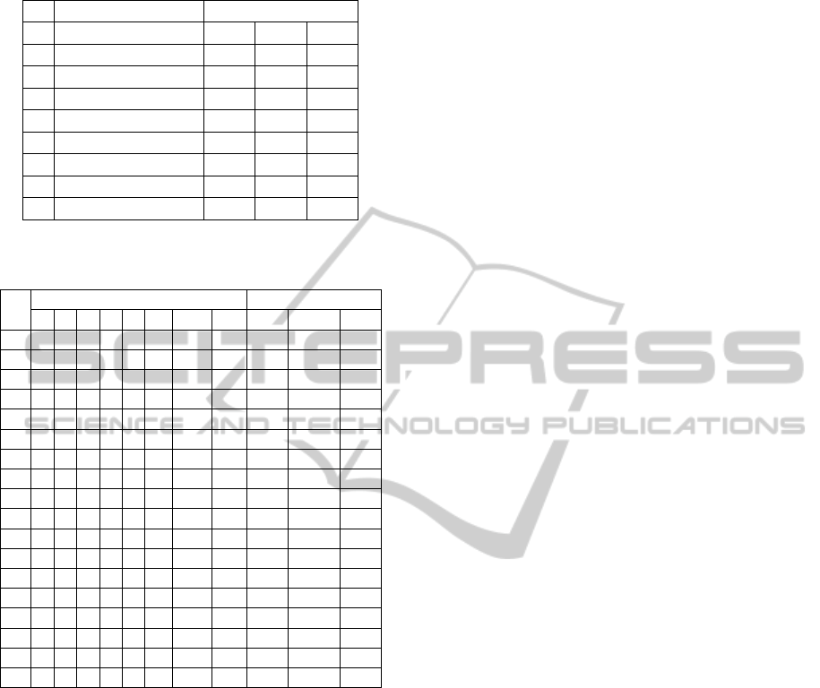
Table 1: Parameter levels.
Levels
Parameters 1 2 3
A Core diameter (%) 48 50 -
B Flute angle (
o
) 38 45 50
C Rake angle (
o
) 18 20 22
D Relief angle 1
st
(
o
) 20 22 25
E Relief angle 2
n
d
(
o
) 25 28 30
F Cutting depth (mm) 0.5 1.0 1.5
G Cutting speed (rpm) 5000 6000 7000
H Feed (mm/flute) 0.05 0.08 0.10
Table 2: Parameter design according to L
18
(2
1
x3
7
)
orthogonal array and performance measures.
No.
Columns Perform. Measures
A B C D E F G H R
a
R
y
R
z
1 48 38 18 20 25 0.5 5000 0.05 0.08 0.93 0.73
2 48 38 20 22 28 1.0 6000 0.08 0.17 1.27 1.17
3 48 38 22 25 30 1.5 7000 0.10 0.18 1.30 1.07
4 48 45 18 20 28 1.0 7000 0.10 1.66 5.73 6.83
5 48 45 20 22 30 1.5 5000 0.05 0.12 1.47 0.90
6 48 45 22 25 25 0.5 6000 0.08 0.19 2.10 1.13
7 48 50 18 22 25 1.5 6000 0.10 0.22 1.80 1.27
8 48 50 20 25 28 0.5 7000 0.05 1.33 12.13 7.10
9 48 50 22 20 30 1.0 5000 0.08 0.19 1.27 1.27
10 50 38 18 25 30 1.0 6000 0.05 0.13 1.20 0.93
11 50 38 20 20 25 1.5 7000 0.08 0.19 1.47 1.23
12 50 38 22 22 28 0.5 5000 0.10 0.17 1.27 1.10
13 50 45 18 22 30 0.5 7000 0.08 0.11 1.03 1.10
14 50 45 20 25 25 1.0 5000 0.10 0.13 1.27 1.03
15 50 45 22 20 28 1.5 6000 0.05 0.14 0.77 0.70
16 50 50 18 25 28 1.5 5000 0.08 0.22 1.37 1.10
17 50 50 20 20 30 0.5 6000 0.10 0.15 1.20 0.97
18 50 50 22 22 25 1.0 7000 0.05 0.16 1.37 0.90
4 MODELLING FRAMEWORK
In the frame of this modelling work a NN was
developed in order to predict the surface roughness
parameters (R
a
, R
y
, and R
z
) during end milling on
the surface texture of Al alloy 5083. The eight (8)
factors studied were used as input parameters of the
NN model.
The 18 experimental data samples (Table 2),
were separated into three groups, namely the
training, the validation and the testing samples.
Training samples are presented to the network
during training and the network is adjusted
according to its error. Validation samples are used to
measure network generalization and to halt training
when generalization stops improving. Testing
samples have no effect on training and so provide an
independent measure of network performance during
and after training (confirmation runs).
Nine (9) samples (50%) were used for training,
four (4) samples (20%) for validation and five (5)
samples (30%) for testing purposes. The samples
that were used for ANN training were selected
following the L
9
Taguchi orthogonal array (i.e.
experiments 1-3, 7-9, and 13-15). For the validation
process were used the samples 4, 12, 16, and 18. The
remaining ones (i.e. 5-6, 10-11, and 17) were used
for testing purposes.
There are many possible types of architecture for
ANN. In this work, the feed-forward with back-
propagation learning (FFBP) architecture has been
selected to predict the surface roughness. These
types of networks have an input layer of X inputs,
one or more hidden layers with several neurons and
an output layer of Y outputs. In the selected ANN,
the transfer function of the hidden layer is
hyperbolic tangent sigmoid, while for the output
layer a linear transfer function was used. The input
vector consists of the eight process parameters of
Table 2. The output layer consists of the
performance measures, namely the R
a
, R
y
and R
z
. In
order to compute the best number of neurons and
hidden layers, several trial and errors have taken
place for the initial learning phase. It was found that
network architecture (8-7-5-4-3) with three hidden
layers of seven (7) neurons in the first hidden layer,
five (5) neurons in the second hidden layer and four
(4) neurons in the third hidden layer exhibits a
minimal error between the output values estimated
by the NN and the data samples provided by the
experimental data.
Back-propagation NNs are prone to the
overtraining problem that could limit their
generalization capability (Tzafestas et al., 1996).
Overtraining usually occurs in ANNs with a lot of
degrees of freedom (Prechelt, 1998) and after a
number of learning loops, in which the performance
of the training data set increases, while the
performance of the validation data set decreases.
The performance of the network is measured by
the MSE of the estimated output with regards to the
values of the experimental data. Mean Squared Error
is the average squared difference between network
output values and target values. Lower values are
better. Zero means no error. The best validation
performance is equal to 0.0069 when the training of
the ANN stops, which means very good network
efficiency. Another performance measure for the
network efficiency is the regression (R). Regression
values measure the correlation between output
values and targets. The acquired results show a very
SURFACE ROUGHNESS MODELLING AND OPTIMIZATION IN CNC END MILLING USING TAGUCHI DESIGN
AND NEURAL NETWORKS
597

good correlation between output values and targets
during training (R=1), validation (R=0.89) and
testing procedure (R=0.93).
Ry (μm)
R
y
vs. Cuttin
g
speed & Feed
(Core diameter = 50 %, Flute angle = 38
o
, Rake angle = 22
o
, Relief angle 1
st
= 22
o
,
Relief angle 2
nd
= 30
o
, Cutting depth = 1,5 mm)
Figure 3: Response surface diagram of R
y
in relation to the
cutting speed and feed, while cutting depth is 1,5 mm.
The trained NN model can be used for the
optimization of the surface roughness parameters
during CNC end milling. This can be done by testing
the behaviour of the response variables (R
a
, R
y
and
R
z
) under different variations in the values of
geometry and cutting parameters. In order to ensure
accurate prediction of the surface roughness
parameters, the values concerning the eight input
parameters should be inside the range of values that
are defined during the experimental setup.
Figure 3 presents an example of a surface
response diagram for the roughness parameter R
y
while cutting speed and feed rate vary within their
range of values. In this diagram all the geometry
parameters were kept constant at their optimum
values. This figure shows that when the cutting
speed increases, as well as in the case of feed rate
reduction, the response variable (surface roughness,
R
y
) decreases.
5 CONCLUSIONS
A FFBP-NN model was built to estimate the surface
roughness indicator response according to the
geometry and cutting parameters of the process. The
performance of the network was found to be
efficient providing very good correlation between
outputs and targets during training (R=1), validation
(R=0.89) and testing procedure (R=0.93).
Furthermore, the response surface diagram in
Figure 3 shows that when the geometry parameters
take their optimum values, the increase of cutting
speed, as well as the decrease of feed rate, results in
deduction of the surface roughness, which is also in
accordance with the machining theory. Multi-
parameter investigation of the process according to
other quality indicators will be studied and analyzed
in future work.
ACKNOWLEDGEMENTS
In memory of George Petropoulos, Assistant
Professor in Machining Processes Technology,
Department of Mechanical & Industrial Engineering,
University of Thessaly, Volos, Greece.
REFERENCES
Chryssolouris, G., Pappas, M., Karabatsou, V., 2004.
Posture based discomfort modeling using neural
networks. Proceedings of IFAC MIM'04, Athens,
Greece, 19–23.
Engin, S., Altintas, Y., 2001. Mechanics and dynamics of
general milling cutters: Part I: helical end mills. Int. J.
Mach. Tools Manu. 41(15), 2195-2212.
Kechagias, J., Iakovakis, V., 2009. A neural network
solution for LOM process performance. Int. J.
Advanced Manufacturing Technology, 43(11–12),
1214–1222.
Kechagias J., Pappas, M., Karagiannis, S., Petropoulos,
G., Iakovakis, V., Maropoulos, S., 2010. An ANN
Approach on the Optimization of the Cutting
Parameters During CNC Plasma-Arc Cutting,
Proceedings of ASME ESDA 2010, Istanbul, Turkey.
Kechagias, J., Petropoulos, G., Iakovakis, V., Maropoulos,
S., 2009. An investigation of surface texture
parameters during turning of a reinforced polymer
composite using design of experiments and analysis.
Int. J. Experimental Design and Process Optimisation.
1(2/3), 164-177.
Markopoulos, A., et al., 2006. Artificial neural networks
modeling of surface finish in electro-discharge
machining of tool steels. Proceedings of ASME ESDA
2006, Torino, Italy.
Phadke, M. S., 1989. Quality Engineering using Robust
Design. Prentice-Hall, Englewood Cliffs, NJ.
Prechelt, L., 1998. Automatic early stopping using cross
validation: quantifying the criteria. Neural Networks,
11(4), 761–767.
Tzafestas, S. G., et al., 1996. On the overtraining
phenomenon of backpropagation NNs. Mathematics
and Computers in Simulation, 40, 507-521.
Yun, W. S., Cho, D. W., 2000. An improved method for
the determination of 3D cutting force coefficients and
runout parameters in end milling. Int. J. Adv. Manuf.
Technol., 16, 851–858.
ICAART 2011 - 3rd International Conference on Agents and Artificial Intelligence
598