AN ADAPTIVE SELECTIVE ENSEMBLE FOR DATA STREAMS

CLASSIFICATION

Valerio Grossi

Department of Pure and Applied Mathematics, University of Padova, via Trieste 63, Padova, Italy

Franco Turini

Department of Computer Science, University of Pisa, largo B. Pontecorvo 3, Pisa, Italy

Keywords:

Data Mining, Data Streams Classiﬁcation, Ensemble Classiﬁer, Concept Drifting.

Abstract:

The large diffusion of different technologies related to web applications, sensor networks and ubiquitous

computing, has introduced new important challenges for the data mining community. The rising phenomenon

of data streams introduces several requirements and constraints for a mining system. This paper analyses a

set of requirements related to the data streams environment, and proposes a new adaptive method for data

streams classiﬁcation. The outlined system employs data aggregation techniques that, coupled with a selective

ensemble approach, perform the classiﬁcation task. The selective ensemble is managed with an adaptive

behavior that dynamically updates the threshold value for enabling the classiﬁers. The system is explicitly

conceived to satisfy these requirements even in the presence of concept drifting.

1 INTRODUCTION

The rapid diffusion of brand new technologies, such

as smartphones, netbooks, sensor networks, related

to communication services, web and safety applica-

tions, has introduced new challenges in data manage-

ment and mining. In these scenarios data arrives on-

line, at a time-varying rate creating the so-called data

stream phenomenon. Conventional knowledge dis-

covery tools cannot manage this overwhelming vol-

ume of data. The nature of data streams requires the

use of new approaches, which involve at most one

pass over the data, and try to keep track of time-

evolving features, known as concept drifting.

Ensemble approaches are a popular solution for

data streams classiﬁcation (Bifet et al., 2009). In these

methods, classiﬁcation takes advantage of multiple

classiﬁers, extracting new models from scratch and

deleting the out-of-date ones continuously. In (Grossi

and Turini, 2010; Grossi, 2009), it was stressed that

the number of classiﬁers actually involved in the clas-

siﬁcation task cannot be constant through time. In the

cited works, it was demonstrated that a selective en-

semble which, based on current data distribution, dy-

namically calibrates the set of classiﬁers to use, pro-

vides a better performance than systems using a ﬁxed

set of classiﬁers constant through time. In our for-

mer approach, the selection of the models involved in

the classiﬁcation step was chosen by a ﬁxed activa-

tion threshold. This choice is the right solution if it

is possible to study a-priori what is the best value to

assign to the threshold. Unfortunately, in many situa-

tions, this information is unavailable, since the stream

data behaviour cannot be modeled. In several real do-

mains, such as intrusion detection, data distribution

can remain stable for a long time, changing radically

when an attack occurs.

This work presents an evolution of the system out-

lined in (Grossi and Turini, 2010; Grossi, 2009). The

new approach introduces a complete adaptive behav-

iuor in the management of the threshold required for

the selection of the set of models actually involved

in the classiﬁcation. The main contribution of this

work is to introduce an adaptive approach for varying

the value of the model activation threshold through

time, inﬂuencing the overall behaviour of the ensem-

ble classiﬁer, based on data change reaction. Our ap-

proach is explicitly explained with the use of binary

attributes. This choice can be seen as a limitation, but

it is worth observing that every nominal attribute can

be easily transformed into a set of binary ones. The

only inability is the direct treatment of numerical val-

136

Grossi V. and Turini F..

AN ADAPTIVE SELECTIVE ENSEMBLE FOR DATA STREAMS CLASSIFICATION.

DOI: 10.5220/0003183501360145

In Proceedings of the 3rd International Conference on Agents and Artiﬁcial Intelligence (ICAART-2011), pages 136-145

ISBN: 978-989-8425-40-9

 2011 SCITEPRESS (Science and Technology Publications, Lda.)

ues. Fortunately, (Gama and Pinto, 2006) represents

a general approach to solve the online discretization

of numerical attributes. The proposed method is par-

ticularly suitable in our context, since it proposes a

discretization method based on two layers. The ﬁrst

layer summarizes data, while the second one con-

structs the ﬁnal binning. The process of updating the

ﬁrst layer works online and requires a single scan over

the data.

Paper Organization: Section 2 introduces our refer-

ence scenario. It outlines some requirements that a

system working on streaming environments should

satisfy. Section 3 describes our approach in details,

highlighting how the requirements introduced in Sec-

tion 2.1 are veriﬁed by the proposed model. Further-

more, it present how our adaptive selection is imple-

mented. In Section 4, we present a comparative study

to understand how the new adaptive approach guaran-

tees a higher reliability of the system. In this section,

our approach is also compared with other well-know

approaches available in the literature. Finally, Section

5 draws the conclusions and introduces some future

works.

2 DATA STREAMS

CLASSIFICATION

Data streams represent a new challenge for the data

mining community. In a stream scenario, traditional

mining methods are further constrained by the unpre-

dictable behaviour of a large volume of data. The

latter arrives on-line at variable rates, and once an

element has been processed, it must be discarded or

archived. In either cases, it cannot be easily retrieved.

Mining systems have no control over data generation,

and they must be capable of guaranteeing a near real-

time response.

Deﬁnition 1. A data stream is an inﬁnite set of el-

ements X = X

,...,X

,... where each X

∈ X has

a + 1 dimensions, (x

,...x

,y), and where y ∈ {⊥

,1,... ,C}, and 1,. . . ,C identify the possible values in

a class.

A stream can be divided into two sets based on

the availability of class label y. If value y is available

in the record (y 6=⊥), it belongs to the training set.

Otherwise the record represents an element to clas-

sify, and the true label will only be available after an

unpredictable period of time.

Given Deﬁnition 1, the notion of concept drift-

ing can be easily deﬁned. As reported in (Klinken-

berg, 2004), a data stream can be divided into batches,

namely b

,...,b

. For each batch b

, data is in-

dependently distributed w.r.t. a distribution P

(). De-

pending on the amount and type of concept drifting,

() will differ from P

i+1

(). A typical example is

customers’ buying preferences, which can change ac-

cording to the day of the week, inﬂation rate and/or

availability of alternatives. Two main types of con-

cept drifting are usually distinguished in the literature,

i.e. abrupt and gradual. Abrupt changes imply a rad-

ical variation of data distribution from a given point

in time, while gradual changes are characterized by a

constant variation during a period of time. The con-

cept drifting phenomenon involves data expiration di-

rectly, and forces stream mining systems to be con-

tinuously updated to keep track of changes. This im-

plies making time-critical decisions for huge volumes

of high-speed streaming data.

2.1 Requirements

As introduced in Section 2, the stream features inﬂu-

ence the development of a data streams classiﬁer rad-

ically. A set of requirements must be taken into ac-

count before proposing a new approach. These needs

highlightseveral implementationdecisions inserted in

our approach.

Since data streams can be potentially unbounded

in size, and data arrives at unpredictable rates, there

are rigid constraints on time and memory required by

a system through time:

Req. 1: the time required for processing every sin-

gle stream element must be constant, which im-

plies that every data sample can be analyzed al-

most only once.

Req. 2: the memory needed to store all the statistics

required by the system must be constant in time,

and it cannot be related to the number of elements

analyzed by the system.

Req. 3: the system must be capable of updating their

structures readily, working within a limited time

span, and guaranteeing an acceptable level of re-

liability.

Given Deﬁnition 1, it is clear that the elements to clas-

sify can arrive in every moment during the data ﬂow.

Req. 4: the system must be able to classify unseen

elements every time during its computation.

Req. 5: the system should be able to manage a set of

models that do not necessarily include contiguous

ones, i.e. classiﬁers extracted using adjacent parts

of the stream.

AN ADAPTIVE SELECTIVE ENSEMBLE FOR DATA STREAMS CLASSIFICATION

137

2.2 Related Work

Mining data streams has rapidly become an important

and challenging research ﬁeld. As proposed in (Gaber

et al., 2005), the available solutions can be classi-

ﬁed into data-based and task-based ones. In the for-

mer approaches a data stream is transformed into an

approximate smaller-size representation, while task-

based techniques employ methods from computa-

tional theory to achieve time and space efﬁcient solu-

tions. Aggregation (Aggarwal et al., 2003; Aggarwal

et al., 2004a; Aggarwal et al., 2004b; Lin and Zhang,

2008), sampling (Domingos and Hulten, 2001) or

summarized data structure, such as histograms (Guha

et al., 2001; Gilbert et al., 2002), are popular example

of data-based solutions. On the contrary, approxima-

tion algorithms approaches such as those introduced

in (Gama et al., 2006; Domingos and Hulten, 2001)

are examples of task-based techniques.

In the context of data streams classiﬁcation, two

main approaches can be outlined, namely instance se-

lection and ensemble learning. Very Fast Decision

Trees (VFDT) (Domingos and Hulten, 2000) with its

improvements (Hulten et al., 2001; Gama and Pinto,

2006; Pfahringer et al., 2008) for concept drifting re-

action and numerical attributes managing represent

examples of instance selection methods. In particular,

the Hoeffding bound guarantees that the split attribute

chosen using n examples, is the same with high proba-

bility as the one that would be chosen using an inﬁnite

set of examples. Last et al. (Cohen et al., 2008) pro-

pose another strategy using an info-fuzzy technique to

adjust the size of a data window. Ensemble learning

employs multiple classiﬁers, extracting new models

from scratch and deleting the out-of-date ones con-

tinuously. Online approaches for bagging and boost-

ing are available in (Oza and Russell, 2001; Chu and

Zaniolo, 2004; Bifet et al., 2009). Different methods

are available in (Street and Kim, 2001; Wang et al.,

2003; Scholz and Klinkenberg, 2005; Kolter and Mal-

oof, 2007; Folino et al., 2007), where an ensemble

of weighted-classiﬁers, including an adaptive genetic

programming boosting, as in (Folino et al., 2007), is

employed to cope with concept drifting. None of the

two techniques can be assumed to be more appro-

priate than the other. (Bifet et al., 2009) provides a

comparison between different techniques not only in

terms of accuracy, but also including computational

features, such as memory and time required by each

system. By contrast, our approach proposes an en-

semble learning that differs from the cited methods

since it is designed to concurrently manage different

sliding windows, enabling the use of a set of classi-

ﬁers not necessarily contiguous and constant in time.

x y z

class value

0 1 1

0 1 0

yes

0 1 1

1 1 1

yes

1 0 0

yes

1 0 1

1 1 1

yes

0 0 0

ind

0 0 1

yes

0 0 0

ind

(a) A stream chunk of 10 ele-

ments

(

,2,3) (

,3,2)

yes

(

,2,1) (

,0,3)

(

,2,0) (

,2,0)

ind

(b) The resulting snapshot

Figure 1: From data stream (a) to snapshot (b).

3 ADAPTIVE SELECTIVE

ENSEMBLE

A detailed description of our system is available in

(Grossi and Turini, 2010; Grossi, 2009). In the

following subsections, we brieﬂy introduce only the

main concepts of our approach highlighting the re-

lations between the requirements outlined in Section

2.1 and the aggregate structures introduced. The pro-

posed structures are primarily conceived to capture

evolving data features, and guarantee data reduction

at the same time. Unfortunately, ensuring a good

trade-off between data reduction, and a powerful rep-

resentation of all the evolving data factors is a non-

trivial task.

3.1 The Snapshot

The snapshot deﬁnition implies the na¨ıve Bayes clas-

siﬁer directly. In our model, the streaming training

set is partitioned into chunks. Each data chunk is

transformed into an approximate more compact form,

called snapshot.

Deﬁnition 2 (Snapshot). Given a data chunk of k el-

ements, with A attributes and C class values, a snap-

shot computes the distribution of the values of at-

tribute a ∈ A with class value c, considering the last k

elements arrived:

:C × A 7→ freq



a,k, c



, ∀a ∈ A,c ∈ C

The following properties are directly derived from

Deﬁnition 2.

ICAART 2011 - 3rd International Conference on Agents and Artificial Intelligence

138

Property 1. Given a stream with C class values and

A attributes, a snapshot is a set of C × A tuples.

Property 2. Building a snapshot S

requires k ac-

cesses to the data stream. Every element is accessed

only once. Computing a snapshot is linear to the k

number of elements.

Figure 1 shows an example of snapshot creation. The

latter implies only a single access to every stream ele-

ment. A snapshot is built incrementally accessing the

data one by one, and updating the respective counters.

Properties 1 and 2 guarantee that a snapshot requires

a constant time and memory space, satisfying require-

ments 1 and 2.

3.1.1 Snapshots of Higher Order

The only concept of snapshot is not sufﬁcient to guar-

antee all the features needed for data managing and

drift reaction. The concept of high-order snapshot is

necessary to maximize data availability for the mining

task guaranteeing only one data access.

Deﬁnition 3 (High-Order snapshot). Given an order

value i > 0, a high-order snapshot, is obtained by

summing h snapshots of i− 1 order:

h×k

∑

j=1

i−1

k, j

∑

j=1



freq



a,k, c



i−1

, ∀a ∈ A,c ∈ C

where, given a class value c and an attribute a,



freq



a,k, c



i−1

refers to the distribution of the val-

ues of attribute a with class value c of the j-th snap-

shot of order i− 1.

Figure 2 shows the relation between snapshots and

their order. The aim is to employ a set of snapshots

created directly from the stream to build new ones,

representingincreasingly larger data windows,simply

by summing the frequencies of their elements.

A high-order snapshot satisﬁes Property 1, since

it has the same structure of a basic one. Moreover,

it further veriﬁes requirements 3, since the creation

of a new high-order snapshot is linear in the number

of attributes and class values. Finally, the creation of

high-order snapshots does not imply any loss of in-

formation. This aspect guarantees that a set of differ-

ent size sliding windows can be simultaneously man-

aged by accessing data stream only once, enabling the

approach to consider every window as computed di-

rectly from the stream.

From a snapshot, or a high-order one, the system

extracts an approximated decision tree, or employs

the snapshot as na¨ıve Bayes classiﬁer directly.

3.2 The Frame

Snapshots are stored to maximize the number of el-

ements for training classiﬁers. A model mined from

a small set of elements tends to be less accurate than

the one extracted from a large data set. If this ob-

servation is obvious in “traditional” mining contexts,

where training sets are accurately built to maximize

the model reliability, in a stream environment this is

not necessarily true. Due to concept drifting, a model

extracted from a large set of data can be less accu-

rate than the one mined from a small training set.

The large data set can include mainly out-of-date con-

cepts.

Snapshots are then stored and managed, based on

their order, in a structure called frame. The order of a

snapshot deﬁnes its level of time granularity. Concep-

tually similar to Pyramidal Time Frame introduced by

Aggarwal et al. in (Aggarwal et al., 2003) and inher-

ited by logarithmic tilted-time window, our structure

sorts snapshots based on the number of elements from

which a snapshot was created.

Deﬁnition 4 (Frame). Given a level value i, and a

level capacity j, a frame is a function that, given a

pair of indexes (x,y) returns a snapshot of order x and

position y:

i, j

: (x, y) 7→ Snapshot

x,y

where: x ∈ {0,...,i− 1} and y ∈ {0,..., j − 1}.

As shown in Figure 3, level 1 contains snapshots

created directly from the stream. Upper levels use the

snapshots of the layer immediately lower to create a

new one. The maximum number of snapshots avail-

able in the frame is constant in time and is deﬁned

by the number of levels and the level capacity. For

each layer, the snapshot are stored with FIFO policy.

The frame memory occupation is constant in time and

is linear with the number of snapshots storable in the

structure.

3.3 Ensemble Management

The concepts introduced in Section 3.1 and 3.2 are

employed to deﬁne and manage an ensemble of clas-

siﬁers. The selective ensemble management can be

brieﬂy described as a four phase approach:

1. For each snapshot S

, a triple (C

) represent-

ing the classiﬁer, its weight and the classiﬁer en-

abling variable b

is extracted from S

2. Since data distribution can change through time,

the models currently in the structure are re-

weighed with the new data distribution, using a

test set of complete data taken from the last por-

tion of the stream directly.

AN ADAPTIVE SELECTIVE ENSEMBLE FOR DATA STREAMS CLASSIFICATION

139

i,1

,. . .,e

i,k

| {z }

k, j

i+1,1

,. . .,e

i+1,k

| {z }

k, j+1

| {z }

2k, j

i+2,1

,. . .,e

j+2,k

| {z }

k, j+2

i+3,1

,. . .,e

i+3,k

| {z }

k, j+3

| {z }

2k, j+1

| {z }

4k, j

.. . e

n,1

,. . .,e

n,k

| {z }

k,n

n+1,1

,. . .,e

n+1,k

| {z }

k,n+1

.. .

Figure 2: Snapshots and their order.

level

k, j+2

k, j+1

k, j

2k,l+2

2k,l+1

2k,l

4k,g+2

4k,g+1

4k,g

...

i S

i−1

k,n+2

i−1

k,n+1

i−1

k,n

Figure 3: The frame structure.

3. Given a level i, every time a new classiﬁer is gen-

erated, the system decides if the new model must

be inserted in the ensemble based on new data dis-

tribution. Apart from the lowest level, where the

new one is inserted in any case, the system selects

the k

most promising models, based on the cur-

rent weight associated to the classiﬁers, to clas-

sify the new data distribution from k

+ 1 models

correctly.

4. Finally, a set of active models is selected, setting

the boolean value b

associated with a C

as true.

The set of active models is selected based on the

value of an activation threshold θ. All the classi-

ﬁers that differ at most θ to the best classiﬁer with

the highest weight are enabled.

The deﬁned approach satisﬁes requirements 4 and 5,

since it can classify a new instance every time it is

required, and can employ a set of not necessarily con-

tiguous classiﬁers, since it is not necessarily true that

every classiﬁer generated through time enters the en-

semble, but even in that case it can be disabled.

Figure 4 shows the overall organization of our ap-

proach. Essentially, for each level in the frame struc-

ture we have a corresponding level in the ensemble.

The subdivision of the data aggregation task from the

mining aspects makes our approach suitable in dis-

tributed/parallel environments as well. One or more

components can be employed to manage the concepts

of snapshot and frame, while another can manage the

ensemble classiﬁer.

3.4 Adaptive Behaviour

As proposed in Section 3.3 our approach has two key

factors inﬂuencing its behavior, the weight measure

to employ and the selection of the θ value. If in the

literature, several weight measures, mainly related to

classiﬁer accuracy, are available and guarantee a good

reliability of the system, the θ threshold represents the

real key factor for the quality of our approach.

In our experiments (Grossi, 2009), we noticed that

the reliability of the system is heavily inﬂuenced by

the θ value. As we shall present in Section 4.3, in-

dependently from the data set employed, activation

values which are too high (or too small) decrease the

predictive power of the ensemble. On the one hand, in

case of relatively stable data, small activation thresh-

old values limit the use of a large set of classiﬁers.

On the contrary, large threshold values damage the se-

lective ensemble in the case of concept drifts. In the

cited experiments, the θ value was ﬁxed by the user

and it did not change through time. Only our experi-

ence and the experimental results drove the selection

of the right value.

The main contribution of this work is to introduce

an adaptive approach into our system. In particular,

we introduce a new approach for varying the value of

the activation threshold through time, thus inﬂuencing

the overall behaviour of the entire system, based on

data change reaction.

The basic idea of the adaptive approach is similar

to the additive-increase/multiplicative-decrease algo-

rithm adopted by TCP Internet protocol for managing

the transfer rate value used in TCP congestion avoid-

ance.

The pseudo-code of the method for managing the

activation threshold is proposed in Figure 5. The

idea behind the algorithm is quite simple. When the

ﬁrst model is inserted in the structure, the activation

threshold and the number of active models are ini-

tialized (Steps 1-5). Successively, every time a new

model is inserted in the ensemble, the procedure at

Step 6 computes how many models will be activated

with the current θ value. If the number of models po-

tentially activatable is higher than the old one (Step

ICAART 2011 - 3rd International Conference on Agents and Artificial Intelligence

140

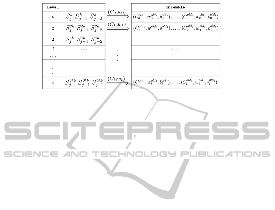
Figure 4: The overall system architecture.

Activation Threshold Algorithm

1: if (oneModel() = true) then

2: θ ← 0.00; activation threshold initialized

oldActModels

← 1

4: return

5: end if

actModels

← getActiveModel(θ)

7: if (

actModels

oldActModels

) then

8: θ ← θ + 0.01; increment threshold value

9: else if (

actModels

oldActModels

) then

10: θ ← θ div 2; decrement threshold value

11: end if

12:

oldActModels

← actModels

13: return

Figure 5: Pseudo-code of the activation threshold algo-

rithm.

7), the threshold is increased. This situation can hap-

pen, when the data distribution remains stable and the

new inserted model is immediately enabled (Step 7-

8). Increasing the threshold value, we can obtain a

better exploitation of the ensemble. On the contrary,

if the number of active models decreases from the pre-

vious invocation, the threshold has to be decreased.

It is useless and dangerous to maintain the current

value, since a data change might be in progress (Step

9-10). It is worth observing that, if the number of

models does not change between the two invocations,

the threshold does not change, since there is no evi-

dence of model improving or data change.

From a computational point of view the algorithm

does not introduce appreciable overhead. Only the

getActiveModel() procedure requires to access the en-

semble structure. If we consider n as the number of

classiﬁers storable in the ensemble, the complexity of

the algorithm is linear in O(n).

The experimental section demonstrates that our

system is no more heavilyinﬂuenced by θ value, since

it changes automatically, adapting it to data distribu-

tion.

4 COMPARATIVE

EXPERIMENTAL EVALUATION

4.1 Data Sets

Several synthetic data sets were introduced in our ex-

periments. This kind of data enables an exhaustive in-

vestigation about the reliability of the stream systems

involving different scenarios. The data behaviour can

be described exactly, characterizing the number of

concept drifts, the rate between a change to another

and the number of irrelevant attributes, or the percent-

age of noisy data.

LED24: Proposed by Breiman et al. in (Breiman

et al., 1984), this generator creates data for a display

with 7 LEDs. In addition to the 7 necessary attributes,

17 irrelevant boolean attributes with random values

are added, and 10 percent of noise is introduced, to

make the solution of the problem harder. This type of

data generates only stable data sets.

Stagger: Introduced by Schlimmer and Granger

in (Schlimmer and Granger, 1986), this prob-

lem consists of three attributes, namely

colour

∈

{green, blue, red},

shape

∈ {triangle, circle,

rectangle}, and

size

∈ {small, medium, large},

and a class

∈ {0, 1}. In its original formulation,

the training set includes 120 instances and consists

of three target concepts occurring every 40 instances.

The ﬁrst set of data is labeled according to the con-

cept

color

= red ∧

size

= small, while the others

include

color

= green ∨

shape

= circle and

size

= medium ∨

size

= large. For each training in-

stance, a test set of 100 elements is randomly gener-

ated according to the current concept.

cHyper: Introduced in (Chu and Zaniolo, 2004),

geometrically, a data set is generated by using a

n-dimensional unit hypercube, and an example x is a

AN ADAPTIVE SELECTIVE ENSEMBLE FOR DATA STREAMS CLASSIFICATION

141

vector of n-dimensions x

∈ [0,1]. The class boundary

is a hyper-sphere of radius r and center c. Concept

drifting is simulated by changing the c position by a

value ∆ in a random direction. This data set generator

introduces noise by randomly ﬂipping the label of a

tuple with a given probability. Two additional data

sets, namely

Hyper

and

Cyclic

are generated using

this approach.

Hyper

does not consider any drifts,

while

Cyclic

proposes the problem of periodic

recurring concepts.

The features of the data sets actually employed are

reported in Table 1. The stable

LED24

and

Hyper

are

useful for testing whether the mechanism for change

reaction has implications for the reliability of the sys-

tems. The evolving data sets test different features of

a stream classiﬁcation system. The

Stagger

problem

veriﬁes, if all the systems can cope with concept drift-

ing, without considering any problem dimensionality.

Then, the problem of learning in the presence of con-

cept drifting is evaluated with the other data sets, also

considering a huge quantity of data with

cHyper

4.2 Systems

Different popular stream ensemble methods are intro-

duced in our experiments. All the systems expect the

data streams to be divided into chunks based on a de-

ﬁned value. All the approaches are implemented in

Java 1.6 with MOA (The University of Waikato, a)

and WEKA libraries (The University of Waikato, b)

for the implementation of the basic learners and em-

ploy complete non-approximate data for the mining

task.

Fix: This approach is the simplest one. It considers

a ﬁxed set of classiﬁers, managed as a FIFO queue.

Every classiﬁer is unconditionally inserted in the en-

semble, removing the oldest one, when the ensemble

is full.

SEA: A complete description and evaluation of this

system can be found in (Street and Kim, 2001). In this

case classiﬁers are not deleted indiscriminately. Their

management is based on a weight measure related to

model reliability. This method represents a special

case of our selective ensemble, where only one level

is deﬁned.

DWM: This system is introduced in (Kolter and Mal-

oof, 2005; Kolter and Maloof, 2007). The approach

implemented here considers a set of data as input to

the algorithm, and a batch classiﬁer as the basic one.

A weight management is introduced, but differently

from SEA, every classiﬁer has a weight associated

with it, when it is created. Every time the classiﬁer

makes a mistake, its weight decreases.

Oza: This system implements the online bagging

method of Oza and Russell (Oza and Russell, 2001)

with the addition of the

ADWIN

technique (Bifet et al.,

2009) as a change detector and as estimator of the

weight of the boosting method.

Single: This approach employs an incremental single

model with EDDM (Gama et al., 2004; Baena-Garcia

et al., 2006) techniques for drift detection. Both Oza

and Single were tested using ASHoeffdingTree and

na¨ıve Bayes models available in MOA.

4.3 Results

All the experiments were run on a PC with In-

tel E8200 DualCore with 4Gb of RAM, employing

Linux Fedora 10 (kernel 2.6.27) as operating system.

Our experiments consider a frame with 8 levels of ca-

pacity 3. Every high-order snapshot is built by adding

2 snapshots. This frame size is large enough to con-

sider snapshots that represent big portions of data at

higher-levels. For each level, an ensemble of 8 classi-

ﬁers was used. The tests were conducted comparing

the use of the na¨ıve Bayes (NB), and the decision tree

(DT) as base classiﬁers. In all the cases, we compare

our Selective Ensemble (SE) (with ﬁxed model acti-

vation threshold set to 0.1 and 0.25) with our Adap-

tive Selection Ensemble ASE. For each data genera-

tor, a collection of 100 training sets (and correspond-

ing test sets) are randomly generated with respect to

the features outlined in Table 1. Every system is run,

and the average accuracy and 95% of interval conﬁ-

dence are reported. Each test consists of a set of 100

observations. All the statistics reported are computed

according to the results obtained.

4.3.1 Results with Stable Data Sets

The results obtained with stable data sets conﬁrm that

the drift detection approach provided by each system

does not heavily inﬂuence its overall accuracy. With

LED24

and

Hyper

problems, all the systems reach a

quite accurate result. Table 2 reports the results ob-

tained with

Hyper

data sets using the na¨ıve Bayes

approach. These results can be compared with the

ones provided in Table 3 in Section 4.3.1, where the

concept drifting problem is added to the same type of

data.

It is worth observing that there are no signiﬁcant

differences between the results obtained by SE ap-

proach, varying the model activation threshold, and

the new ASE approach provides a result in line with

the best ones. These results demonstrate that the

adaptive behavior mechanism does not negatively in-

ﬂuence the reliability of the system in the case of sta-

ICAART 2011 - 3rd International Conference on Agents and Artificial Intelligence

142

Table 1: Description of data sets.

dataSet #inst #attrs #irrAttrs #classes %noise #drifts

LED24

a/b/test

10k / 100k / 25k 24 17 10 10% none

Hyper

a/b/test

10k / 100k / 25k 15 0 2 0 none

Stagger

a/test

1200 / 120k 9 0 2 0 3 (every 400) / (every 40k)

Stagger

b/test

12k / 1200k 9 0 2 0 3 (every 4k) / (every 400k)

cHyper

a/b/c

10k / 100k / 1000k 15 0 2 10% 20 (every 500) / (every 5k) / (every 50k)

cHyper

test

250k 15 0 2 10% 20 (every 12.5k)

Cyclic

600k 25 0 2 5% 15×4 (every 10k)

Cyclic

test

150k 25 0 2 5% 15×4 (every 2.5k)

Table 2: Results using na¨ıve Bayes with the

Hyper

problem.

Hyper

avg std dev conf

ASE 92.74 / 93.93 1.92 / 2.88 0.38 / 0.49

0.1

92.72 / 93.92 2.20 / 2.52 0.43 / 0.50

0.25

92.70 / 93.91 2.22 / 2.53 0.43 / 0.50

Fix

91.82 / 92.35 2.54 / 2.98 0.50 / 0.58

SEA

92.97 / 94.44 1.80 / 1.64 0.50 / 0.32

DWM

91.82 / 92.76 2.12 / 2.74 0.42 / 0.54

Oza

92.39 / 93.73 2.30 / 0.40 0.45 / 0.08

Single 90.04 / 92.68 3.25 / 2.82 0.64 / 0.55

ble data streams. On the contrary, the new approach

enables a better ensemble exploitation.

Moreover, Table 2 highlights that Single model

requires a large quantity of data to provide a good

performance. Finally, Fix

and SEA

provide good

results that, compared with the ones obtained by

the same systems analyzing the

cHyper

and

Cyclic

problems, demonstrate that these kinds of approaches

guarantee appreciable results only with a quite sta-

ble phenomenon. They do not provide a fast reaction

to concept drifting, since the models involved in the

classiﬁcation task are constant in time, and when a

drift occurs, they have to change a large part of the

models, before classifying new concepts correctly.

4.3.2 Results with Evolving Data Sets

Table 3 reports the overall results obtained analyz-

ing the

cHyper

problem, considering both decision

tree and na¨ıve Bayes models. Differently from the

results obtained with stable data sets, it is worth ob-

serving that the active model threshold inﬂuences the

overall results. Varying the value from 0.1 to 0.25,

and especially considering

cHyper

and

cHyper

, SE

system presents a difference even larger than 6% be-

tween the two values. On the contrary, our ASE

approach provides an accuracy in line with the best

value, even considering standard deviation. This de-

mostrates that, without knowing the ideal threshold

value for model activation, our ASE approach rep-

resents the right solution to the different situations

involved in a stream scenario, and simulated by the

three cases of the

cHyper

problem. As stated in the

previous section, it is worth observing the poor perfor-

mances of Fix and SEA in the case of evolving data.

These obsevations are further validated by the results

obtained with the

Stagger

problem, that essentially

follow the ones proposed in Table 3.

Finally, Table 4 outlines the resources required by

the systems. The memory requirements were tested

using NetBeans 6.8 Proﬁler. We can state that Single

requires less memory than ensemble methods, which

need a quantity of memory that is essentially linear

with respect to the number of classiﬁers stored in the

ensemble. The different nature of the two classes

of systems inﬂuences this value. The average mem-

ory required by our system is slightly higher than the

others, since our system manages two different struc-

tures, as suggested at the end of Section 3.3. The run

time behavior conﬁrms this trend. In this case the drift

detection approach inﬂuences the execution time of

a method. Let us compare the bagging method Oza

with respect to DWM, SEA

and ASE. These tests

highlight that incremental single model systems are

faster than ensemble ones, since they have to update

only one model. On the contrary, considering the ac-

curacy, single model systems rarely provide best av-

erage values. Finally, Oza guarantees an appreciable

reliability with every data set, but its execution time

is deﬁnitely higher than the others.

We conclude this section, proposing the results

obtained considering the

Cyclic

problem. The latter

are presented considering the na¨ıve Bayes approach

and analyzing different rates between the chunk size

and the elements to classify. As shown in Figure 6,

even in this case, our ASE approach is in-line with

the SE

0.1

and better than the others. Since this prob-

lem presents recurring concepts, it is worth observing

AN ADAPTIVE SELECTIVE ENSEMBLE FOR DATA STREAMS CLASSIFICATION

143

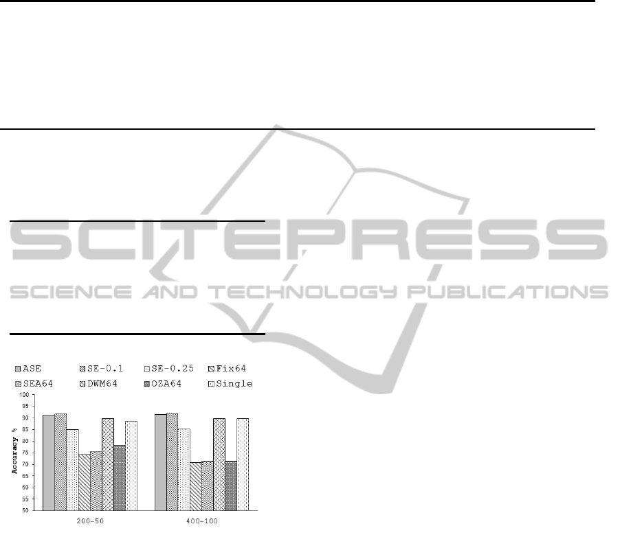
Table 3: Overall results with the

cHyper

problem.

cHyper

- decision tree

cHyper

- na¨ıve Bayes

avg std dev conf avg std dev conf

ASE 83.58 / 88.72 / 93.19 0.51 / 0.40 / 0.28 0.10 / 0.08 / 0.06 87.52 / 92.23 / 95.94 0.38 / 0.43 / 0.33 0.09 / 0.08 / 0.06

0.1

84,05 / 89,43 / 93,09 0,49 / 0,40 / 0,32 0,10 / 0,08 / 0,06 87,62 / 92,62 / 95,98 0,42 / 0,43 / 0,47 0,08 / 0,09 / 0,09

0.25

78,42 / 86,10 / 91,86 0,86 / 0,35 / 0,23 0,17 / 0,07 / 0,23 79,90 / 86,80 / 92,14 0,83 / 0,40 / 0,22 0,16 / 0,08 / 0,22

Fix

70,26 / 82,02 / 90,62 2,58 / 1,23 / 0,13 0,51 / 0,24 / 0,13 73,72 / 83,69 / 94,16 2,60 / 1,35 / 0,40 0,51 / 0,26 / 0,40

SEA

70,26 / 82,14 / 90,04 2,58 / 1,10 / 0,14 0,51 / 0,22 / 0,14 73,72 / 84,23 / 94,78 2,60 / 1,27 / 0,31 0,51 / 0,25 / 0,31

DWM

77,75 / 85,18 / 92,65 1,94 / 0,60 / 0,14 0,38 / 0,04 / 0,14 85,93 / 92,18 / 95,63 1,76 / 0,18 / 0,38 0,35 / 0,04 / 0,38

Oza

81,99 / 89,60 / 92,40 0,97 / 0,37 / 0,25 0,19 / 0,07 / 0,25 80,01 / 87,31 / 89,78 1,23 / 0,54 / 0,56 0,24 / 0,11 / 0,56

Single 81,50 / 87,85 / 89,99 1,60 / 0,70 / 0,34 0,31 / 0,14 / 0,34 81,25 / 89,47 / 93,34 2,02 / 0,87 / 0,84 0,40 / 0,17 / 0,84

Table 4:

cHyper

time and memory required.

decision tree na¨ıve Bayes

avg used run time avg used run time

heap (KB) (sec.) heap (KB) (sec.)

ASE 9276 82,40 7572 27,42

SE 9233 80,80 7894 27,45

Fix

8507 47,54 5317 23,82

SEA

7980 152,07 5371 97,76

DWM

5111 77,56 5137 21,21

Oza

10047 393,93 6664 290,24

Single 5683 11,54 5399 8,26

Figure 6: Average accuracy using na¨ıve Bayes with the

Cyclic

problem.

how our approach can exploit the selective ensemble

better than the others, since some models which are

currently out of context are not deleted by the sys-

tem, but simply disabled. If a concept becomes newly

valid, the model can be reactivated. This behaviour is

still valid, even in the case of the adaptive approach.

5 CONCLUSIONS

The preliminary results show that, with respect to the

use of a ﬁxed threshold, our adaptive algorithm pro-

vides a slightly worst performance than the ones of

the best value of the threshold. Unfortunately, the

choice of the best value is not always feasible, and

if a wrong selection is made, the system loses its pre-

cision. On the contrary, our adaptive approach does

not require any assumption about active model values

and displays good adaptation to the different scenar-

ios. This work represents a ﬁrst step to guarantee a

system completely adaptable to the different stream-

ing factors. As future works, our aims are to test our

adaptive model in a real stream application with real

data. Moreover, we are currently studying the intro-

duction of runtime monitoring tools for automatically

adapting our system, e.g varying the number of frame

levels, or the models available for each layer, dynam-

ically considering memory consumption and time re-

sponse constraints.

REFERENCES

Aggarwal, C. C., Han, J., Wang, J., and Yu, P. (2003).

A framework for clustering evolving data streams.

In Proceedings of the 2003 International Conference

on Very Large Data Bases (VLDB’03), pages 81–92,

Berlin, Germany.

Aggarwal, C. C., Han, J., Wang, J., and Yu, P. (2004a).

A framework for projected clustering of high dimen-

sional data streams. In Proceedings of the 2004 In-

ternational Conference on Very Large Data Bases

(VLDB’04), pages 852–863, Toronto, Canada.

Aggarwal, C. C., Han, J., Wang, J., and Yu, P. (2004b). On

demand classiﬁcation of data streams. In Proceedings

of the 10th International Conference on Knowledge

Discovery and Data Mining (KDD’04), pages 503–

508, Seattle, WA.

Baena-Garcia, M., del Campo-Avila, J., Fidalgo, R., Bifet,

A., Ravalda, R., and Morales-Bueno, R. (2006). Early

drift detection method. In International Workshop on

Knowledge Discovery from Data Streams.

Bifet, A., Holmes, G., Pfahringer, B., Kirby, R., and

Gavald´a, R. (2009). New ensemble methods for evolv-

ing data streams. In Proceedings of the 15th Interna-

tional Conference on Knowledge Discovery and Data

Mining, pages 139–148.

ICAART 2011 - 3rd International Conference on Agents and Artificial Intelligence

144

Breiman, L., Friedman, J., Olshen, R., and Stone, C. (1984).

Classiﬁcation and Regression Trees. Wadsworth Inter-

national Group, Belmont, CA.

Chu, F. and Zaniolo, C. (2004). Fast and light boosting for

adaptive mining of data streams. In Proceedings of the

8th Paciﬁc-Asia Conference Advances in Knowledge

Discovery and Data Mining (PAKDD’04), pages 282–

292, Sydney, Australia.

Cohen, L., Avrahami, G., Last, M., and Kandel, A.

(2008). Info-fuzzy algorithms for mining dynamic

data streams. Applied Soft Computing, 8(4):1283–

1294.

Domingos, P. and Hulten, G. (2000). Mining high-speed

data streams. In Proceedings of the 6th International

Conference on Knowledge Discovery and Data Min-

ing (KDD’00), pages 71–80, Boston. MA.

Domingos, P. and Hulten, G. (2001). A general method

for scaling up machine learning algorithms and its

application to clustering. In Proceedings of the

18th International Conference on Machine Learning

(ICML’01), pages 106–113, Williamstown, MA.

Folino, G., Pizzuti, C., and Spezzano, G. (2007). Mining

distributed evolving data streams using fractal gp en-

sembles. In Proceedings of the 10th European Confer-

ence Genetic Programming (EuroGP’07), pages 160–

169, Valencia, Spain.

Gaber, M. M., Zaslavsky, A., and Krishnaswamy, S. (2005).

Mining data streams: a review. ACM SIGMOD

Records, 34(2):18–26.

Gama, J., Fernandes, R., and Rocha, R. (2006). Decision

trees for mining data streams. Intelligent Data Analy-

sis, 10(1):23–45.

Gama, J., Medas, P., Castillo, G., and Rodrigues, P. (2004).

Learning with drift detection. In SBIA Brazilian Sym-

posium on Artiﬁcial Intelligence, pages 286–295.

Gama, J. and Pinto, C. (2006). Discretization from data

streams: applications to histograms and data min-

ing. In Proceedings of the 2006 ACM symposium on

Applied computing (SAC’06), pages 662–667, Dijon,

France.

Gilbert, A., Guha, S., Indyk, P., Kotidis, Y., Muthukrish-

nan, S., and Strauss, M. (2002). Fast, small-space

algorithms for approximate histogram maintenance.

In Proceedings of the 2002 Annual ACM Symposium

on Theory of Computing (STOC’02), pages 389–398,

Montreal, Quebec, Canada.

Grossi, V. (2009). A New Framework for Data Streams

Classiﬁcation. PhD thesis, Supervisor Prof. Franco

Turini, University of Pisa.

Grossi, V. and Turini, F. (2010). A new selective ensemble

approach for data streams classiﬁcation. In Proceed-

ings of the 2010 International Conference in Artiﬁcial

Intelligence and Applications (AIA’2010), pages 339–

346, Innsbruck, Austria.

Guha, S., Koudas, N., and Shim, K. (2001). Data-

streams and histograms. In Proceedings of the 2001

Annual ACM Symposium on Theory of Computing

(STOC’01), pages 471–475, Heraklion, Crete, Greece.

Hulten, G., Spencer, L., and Domingos, P. (2001). Min-

ing time changing data streams. In Proceedings of the

7th International Conference on Knowledge Discov-

ery and Data Mining (KDD’01), pages 97–106, San

Francisco, CA.

Klinkenberg, R. (2004). Learning drifting concepts: Exam-

ple selection vs. example weighting. Intelligent Data

Analysis, 8:281–300.

Kolter, J. Z. and Maloof, M. A. (2005). Using additive ex-

pert ensembles to cope with concept drift. In Proceed-

ings of the 22nd International Conference on Machine

learning (ICML’05), pages 449–456, Bonn, Germany.

Kolter, J. Z. and Maloof, M. A. (2007). Dynamic weighted

majority: An ensemble method for drifting concepts.

Journal of Machine Learning Research, 8:2755–2790.

Lin, X. and Zhang, Y. (2008). Aggregate computation

over data streams. In Procedings of the 10th Asia

Paciﬁc Web Conference (APWeb’08), pages 10–25,

Shenyang, China.

Oza, N. C. and Russell, S. (2001). Online bagging and

boosting. In Proceedings of 8th International Work-

shop on Artiﬁcial Intelligence and Statistics (AIS-

TATS’01), pages 105–112, Key West, FL.

Pfahringer, B., Holmes, G., and Kirkby, R. (2008). Han-

dling numeric attributes in hoeffding trees. In

Proceeding of the 2008 Paciﬁc-Asia Conference on

Knowledge Discovery and Data Mining (PAKDD’08),

pages 296–307, Osaka, Japan.

Schlimmer, J. C. and Granger, R. H. (1986). Beyond in-

cremental processing: Tracking concept drift. In Pro-

ceedings of the 5th National Conference on Artiﬁcial

Intelligence, pages 502–507, Menlo Park, CA.

Scholz, M. and Klinkenberg, R. (2005). An ensemble

classiﬁer for drifting concepts. In Proceeding of

2nd International Workshop on Knowledge Discovery

from Data Streams, in conjunction with ECML-PKDD

2005, pages 53–64, Porto, Portugal.

Street, W. N. and Kim, Y. (2001). A streaming ensem-

ble algorithm (SEA) for large-scale classiﬁcation. In

Proceedings of the 7th International Conference on

Knowledge Discovery and Data Mining (KDD’01),

pages 377–382, San Francisco, CA.

The University of Waikato. MOA: Mas-

sive Online Analysis, August 2009.

http://www.cs.waikato.ac.nz/ml/moa.

The University of Waikato. Weka 3: Data

Mining Software in Java, Version 3.6.

http://www.cs.waikato.ac.nz/ml/weka.

Wang, H., Fan, W., Yu, P. S., and Han, J. (2003). Mining

concept-drifting data streams using ensemble classi-

ﬁers. In Proceedings of the 9th International Con-

ference on Knowledge Discovery and Data Mining

(KDD’03), pages 226–235, Washington, DC.

AN ADAPTIVE SELECTIVE ENSEMBLE FOR DATA STREAMS CLASSIFICATION

145