
SOLVING NON BINARY CONSTRAINT SATISFACTION
PROBLEMS WITH DUAL BACKTRACKING ON HYPERTREE
DECOMPOSITION
Zineb Habbas, Kamal Amroun
LITA, University Paul-Verlaine of Metz, Metz, France
Department of Computer Sciences, University of Bejaia, Bejaia, Algeria
D
aniel Singer
LITA, University Paul-Verlaine of Metz, Metz, France
Keywords:
CSP, Dual backtracking, Forward-checking, Hypertree decomposition, Structural decomposition, Ordering
Heuristics.
Abstract:
Solving a CSP (Constraint Satisfaction Problem) is NP-Complete in general. However, there are various
classes of CSPs that can be solved in polynomial time. Some of them can be identified by analyzing their
structure. It is theoretically well established that a tree (or hypertree) structured CSP can be solved in a
backtrack-free way leading to tractability. Different methods exist for converting CSPs in a tree (or hypertree)
structured representation. Among these methods Hypertree Decomposition has been proved to be the most
general one for non-binary CSPs. Unfortunately, in spite of its good theoretical bound, the unique algorithm
for solving CSP from itshypertree structure is inefficient in practice due to its memory explosion. To overcome
this problem, we propose in this paper a new approach exploiting a Generalized Hypertree Decomposition.
We present the so called HD
DBT algorithm (Dual BackTracking algorithm guided by an order induced by
a generalized Hypertree Decomposition). Different heuristics and implementations are presented showing its
practical interest.
1 INTRODUCTION
Many important real world problems can be formu-
lated as Constraint Satisfaction Problems (CSPs). The
most usual complete method for solving CSPs is
based on a backtracking search. This approach has an
exponential worst-case time complexity of O(m.d
n
)
for a CSP instance with m the number of constraints,
n the number of variables and d the largest size of
variable domains. Solving a CSP is NP-Complete
in general but there are various classes of CSPs that
can be solved in polynomial time. Freuder (Freuder,
1982) proved that a tree-structured CSP can be solved
efficiently and many efforts have been made to de-
fine tree-like decomposition methods that lead to
tractability. Methods deriving from the Database area
have been successfully used to characterize some new
tractable classes (Jeavons et al., 1994; Gyssens et al.,
1994; Gottlob et al., 2000; Gottlob et al., 2005). Their
main common principle is to decompose the CSP into
a number of subproblems organized in a tree or an hy-
pertree structure. These subproblems are then solved
independently and the solutions are propagated in a
backtrack-free manner to solve the initial CSP as de-
scribed in (Dechter and Pearl, 1989). Numerous other
decomposition methods have been proposed, to cite
some of the most important ones: biconnected com-
ponents (Freuder, 1982), hinge decomposition com-
bined with tree clustering (Gyssens et al., 1994) and
spread-cut decomposition (David Cohen, 2005). A
more recent work (Greco and Scarcello, 2010) pro-
posed a deep study on different versions of structural
decompositions deriving from binary representations
of general (non-binary) CSPs. This study gives a the-
oretical comparison of structural decompositions on
binary representations with direct non-binary ones.
All these methods are characterized by their compu-
tational complexity in terms of the tree (resp. hyper-
tree) width they generate. Among them Gottlob et
al. (Gottlob et al., 2000) have shown the hypertree
146
Habbas Z., Amroun K. and Singer D..
SOLVING NON BINARY CONSTRAINT SATISFACTION PROBLEMS WITH DUAL BACKTRACKING ON HYPERTREE DECOMPOSITION.
DOI: 10.5220/0003184801460156
In Proceedings of the 3rd International Conference on Agents and Artificial Intelligence (ICAART-2011), pages 146-156
ISBN: 978-989-8425-40-9
Copyright
c
2011 SCITEPRESS (Science and Technology Publications, Lda.)

decomposition dominates all the other structural de-
composition methods excepted the methods recently
introduced in (Grohe and Marx, 2006).
Most of works on structural decompositions are
purely theoretical to define new general tractable
classes. However, the main drawback of these ap-
proaches from a practical viewpoint is the memory
space explosion due to the expression of relations as-
sociated to constraints by tables and the storage of all
the solutions resulting from join operations as well.
The representation of relations by tables is adequate
for the Database processing using auxiliary memory
disks to save all the relations, but is not realistic for
solving a CSP which requires to save all the structure
in RAM. This is the main reason why the first basic
algorithm (Gottlob et al., 2001) proposed in the liter-
ature to solve CSP with an hypertree is inefficient in
practice. To use more efficiently the structural decom-
position in the search algorithm, the join and semi-
join operations have to be discarded. This idea has
been introduced by different researchers.
In (Pang and Goodwin, 1997; Pang and Goodwin,
2003) Pang et al. have proposed a w-CBDT algo-
rithm combining both merits of Constraint-Directed
Backtracking and structural decompositions, but the
authors do not consider optimal structural decom-
positions. Jegou et al. (J´egou and Terrioux, 2003)
have introduced the successfull method called BTD
(Backtracking with Tree Decomposition) which is an
enumerative search algorithm guided by some pre-
established order induced by a tree decomposition.
This paper goes forward in the same direction to solve
non-binary CSPs directly using efficiently hypertree
decomposition.
We propose an alternative approach to BTD called
HD DBT for Dual BackTracking algorithm guided
by an order induced by an Hypertree Decomposition.
The main idea of this approach is that search will be
guided for the choice of the partial solution by the hy-
pertree structure. HD DBT is more adapted to solve
non-binary CSPs represented as hypergraphs. Given
a CSP and its hypergraph representation, HD DBT
computes one Hypertree Decomposition and it looks
for a solution by using a dual backtracking search al-
gorithm. We propose and compare different heuristics
to achieve “the best” depth-first traversal of the hyper-
tree decomposition wrt. CSP solving complexity. The
hypertree decomposition properties make the general-
isation of BTD to HD DBT non obvious. Informally,
HD DBT is guided by an order on the clusters of con-
straints and not on the clusters of variables while (as
BTD) the connectivity property concerns the clusters
of variables. MoreoverBTD is based on a tree decom-
position which is complete while HD DBT is based
on hypertree decomposition which is not. Thus be-
fore solving a CSP using an hypertree decomposition
we have to complete the resulting hypertree.
The paper is organized as follows: section 2 gives
the preliminary and necessary notions on CSP and
decomposition methods with a special focus on the
hypertree decomposition which is the most general
one. Section 3 presents the basic algorithm exploit-
ing an hypertree decomposition to solve CSPs. Sec-
tion 4 presents our new HD DBT approach. Sec-
tion 5 gives the first experimental results of HD DBT
compared with the basic algorithm proposed in (Got-
tlob et al., 2001). Then we present an improved
HD DBT+FC implementation together with different
heuristics guiding the resolution. Finally, Section 6
gives a conclusion.
2 PRELIMINARIES
In this section we recall the basic definitions of con-
straint satisfaction problems, hypergraphs, hypertree
and generalized hypertree decompositions.
2.1 Constraint Satisfaction Problems
The notion of Constraint Satisfaction Problems (CSP)
was formally defined by U. Montanari (Montanari,
1974).
Definition 1 (Constraint Satisfaction Problem). A
CSP is defined as a triple P =< X, D,C > where :
X = {x
1
, x
2
, ..., x
n
} is a set of n variables.
D = {d
1
, d
2
, ..., d
n
} is a set of finite domains; each
variable x
i
takes its value in its domain d
i
.
C = {c
1
, c
2
, ..., c
m
} is a set of m constraints. Each
constraint c
i
is a pair (S(c
i
), R(c
i
)) where S(c
i
) ⊆ X,
is a subset of variables, called the scope of c
i
and
R(c
i
) ⊆
∏
x
k
∈S(c
i
)
d
k
is the constraint relation, that
specifies the legal combinations of values.
A solution to a CSP is an assignment of values
to all the variables such that all the constraints
are satisfied. Solving a CSP means to find a so-
lution if it exists. Binary CSPs are those defined
where each constraint involves only two variables
∀i ∈ 1. . . m : |S(c
i
)| = 2.
In order to study the structural properties of a
CSP, we need to present the following definitions.
For more detailed descriptions see eg. (Dechter,
2003), (Gottlob et al., 2001) and (Gottlob et al.,
2002).
SOLVING NON BINARY CONSTRAINT SATISFACTION PROBLEMS WITH DUAL BACKTRACKING ON
HYPERTREE DECOMPOSITION
147

Definition 2 (Hypergraph). A hypergraph is a struc-
ture H =< V, E > that consists of a set of vertices
V and a set of hyperedges E where each hyperedge
h ∈ E is a subset of vertices of V. The hyperedges
differ from edges of graphs in that they may connect
more than two vertices.
The structure of a CSP P=< X, D,C > is entierely
captured by its associated hypergraph H =< V, E >
where the set of vertices V is the set of variables X
and the set of hyperedges E corresponds to the set of
constraints C. For any subset of hyperedges K ⊆ E
let be vars(K) =
S
e∈K
e the set of the variables
occuring in the edges of K. For any subset L ⊆ V
let be edgevars(L) = vars({e|e ∈ E, e ∩ L 6=
/
0}) the
set of all variables occuring in any edge intersecting L.
Definition 3 (Hypertree). Let H =< V, E > be a
hypergraph. A hypertree for hypergraph H is a triple
< T, χ, λ > where T = (N, B) (the sets of nodes and
branche-edges) is a rooted tree and χ and λ are two
labelling functions on nodes of T. The functions χ
and λ map each node p ∈ N on two sets χ(p) ⊆ V
and λ(p) ⊆ E.
A tree is a pair < T, χ > where T = (N, B) is a
rooted tree and χ is a labelling function as previously
defined. T
p
denotes the subtree of T rooted at node p.
Definition 4 (Hypertree decomposition). A hypertree
decomposition of a hypergraph H =< V, E >, is a hy-
pertree < T, χ, λ > which satisfies the following con-
ditions:
1. For each (hyper)edge h ∈ E, there exists p ∈ N
such that vars(h) ⊆ χ(p). We say that p covers h.
2. For each vertex v ∈ V, the set {p ∈ N|v ∈ χ(p)}
induces a (connected) subtree of T.
3. For each node p ∈ N,χ(p) ⊆ vars(λ(p)).
4. For each node p ∈ N, vars(λ(p))
T
χ(T
p
) ⊆ χ(p)
The width of a hypertree decomposition
< T,χ, λ > is max
p∈N
|λ(p)|. The hypertree-
width htw(H ) of a hypergraph H is the minimum
width over all its possible hypertree decompositions.
Definition 5 (Generalized hypertree decomposition).
A generalized hypertree decomposition is a hypertree
which satisfies the first three conditions of the hyper-
tree decomposition (see Definition 4).
The width of a generalized hypertree decompo-
sition < T, χ, λ > is max
p∈N
|λ(p)|. The generalized
a b c
c1
c2
c3
c4
c5
c6
d e
f g h
i
j k
l
An hypergraph H
Its Hypertree Decomposition
htw = 2
{k, j, l}, {c6}
{a, b, c}, {c1}
{f, g, h}, {c4}
{g, i, k}, {c5}
{a, d, f, e, c, h}, {c2, c3}
Figure 1: A hypergraph and one of its hypertree decompo-
sition.
hypertree-width ghw(H ) of a hypergraph H is the
minimum width over all its possible generalized
hypertree decompositions.
Definition 6. A hyperedge h of a hypergraph
H =< V, E > is strongly covered in HD =< T, χ, λ >
if there exists p ∈ N such that all the vertices in h are
contained in χ(p) and h ∈ λ(p).
Definition 7. A hypertree decomposition < T, χ, λ >
of a hypergraph H =< V, E > is a complete hypertree
decomposition if every hyperedge h of H =< V, E >
is strongly covered in HD =< T, χ, λ >.
2.2 Computing an Hypertree
Decomposition
In this section we briefly present the two main ap-
proaches proposed in the literature to compute hy-
pertree decompositions: the exact methods and the
heuristics ones.
2.2.1 Exact Methods
Given a hypergraph H =< V, E >, exact algorithms
aim at finding a hypertree decomposition with width
w less than or equal to a constant k, if such a de-
composition exists. The first exact algorithm named
opt-k-decomp for the generation of an optimal hy-
pertree decomposition is due to Gottlob et al. (Got-
tlob et al., 1999). This algorithm builds a hyper-
tree decomposition in two steps: it finds if a hyper-
graph H =< V, E > has a hypertree decomposition
HD =< T, χ, λ > with width less than or equal to a
constant k. If it is the case it finds a hypertree decom-
position of smallest possible width. The algorithm
opt-k-decomp runs in O(m
2k
V
2
) where m is the num-
ber of hyperedges, V is the number of vertices and k
is a constant.
Among the number of improvements to opt-
k-decomp we can cite Red-k-decomp (Harvey and
ICAART 2011 - 3rd International Conference on Agents and Artificial Intelligence
148

Ghose, 2003) and the Subbarayan and Anderson al-
gorithm (Sathiamoorthy and Andersen, 2007) which
is a backtracking version of opt-k-decomp. How-
ever these exact methods have an important drawback
which is the huge amount of memory space needed
and the bad running time resulting in inefficiency in
practice for large instances. To overcome these lim-
itations some heuristics have been proposed to com-
pute hypertree decompositions.
2.2.2 Heuristics
Heuristics aim at finding a hypertree decomposition
with the smallest possible width (tree-width) but with-
out any theoretical guaranty to succeed. There are
several heuristics to compute a hypertree decomposi-
tion. Korimort (Korimort, 2003) proposed one heuris-
tics based on the vertices connectivity of the given hy-
pergraph. Samer (Samer, 2005) explored the use of
branch decomposition for constructing hypertree de-
compositions. Dermaku et al. (Dermaku et al., 2005)
proposed the following heuristics: BE (Bucket Elim-
ination), DBE (Dual Bucket Elimination) and Hyper-
graph partitioning. Musliu and Schafhauser (Musliu
and Schafhauser, 2005) explored the use of genetic al-
gorithms for generalized hypertree decompositions.
We outline the two successful BE and DBE heuristics
for generating hypertree decompositions.
The Bucket Elimination (BE) Heuristics
(Dechter, 1999) was successfully used to compute
a tree decomposition of a given graph (or a primal
graph of a hypergraph). BE has been extended by
Dermaku et al. (Dermaku et al., 2005) to compute
a hypertree decomposition or more precisely a
generalized hypertree decomposition. The simple
idea behind this extension derives from the fact that
a generalized hypertree decomposition satisfies the
properties of a tree decomposition. Consequently, for
computing a generalized hypertree decomposition,
BE proceeds as follows. First, it builds a tree
decomposition using (basic) BE. Then, it creates
the λ − labels for each node of this tree in order to
satisfy the third condition of generalized hypertree
decomposition according to the Definition 5. This is
done greedily by attempting to cover the variables
of each node by hyperedges. In practice the BE
heuristics requires a good vertices ordering to be
efficient.
The Dual Bucket Elimination (DBE) Heuris-
tics was proposed by Dermaku et al. (Dermaku et al.,
2005). DBE simply applies the BE heuristics on the
dual graph of the hypergraph. The idea behind using
the dual graph structure instead of the primal graph
is that BE minimizes the χ − labels while the width
of a hypertree decomposition is determined by the
λ − labels. This is exactly what is done when apply-
ing BE to the dual graph of the hypergraph.
3 SOLVING CSP USING AN
HYPERTREE
DECOMPOSITION
To solve any CSP using a generalized hypertree de-
composition, the first step consists in computing the
generalized hypertree decomposition either with an
exact or with an heuristic method. The next step trans-
forms the generalized hypertree decomposition into
a complete one in order to cover each constraint by
at least one node of the hypertree. Consequently the
complete generalized hypertree decomposition may
be seen as a join tree of an equivalent (wrt. its so-
lutions) acyclic CSP. Each node of the join tree repre-
sents a subproblem of the new acyclic CSP. The third
step of the resolution is described in algorithm 1 due
to Gottlob et al. (Gottlob et al., 2001). In algorithm 1,
each subproblem is solved independently and it can
be done by a parallel algorithm. The Acyclic solving
algorithm is used for finding a complete consistent so-
lution of the initial CSP.
Algoritm 1: Gottlob Algorithm (Gottlob et al., 2001).
Input: a complete generalized hypertree
decomposition < T, χ, λ > associated to a
given CSP.
Output: a solution A of the CSP if it is satisfiable
begin
σ = {n
1
, n
2
, . . . , n
m
} a node ordering with n
1
the
root of the hypertree and each node precedes all
its sons in σ;
foreach p a node in σ do
R
p
= (⊲⊳
C
j
∈λ(p)
R
j
)[χ(p)] ;
end
for i = m to 2 do
Let v
j
the father of v
i
in σ ;
R
j
= R
j
∝ R
i
;
end
for i = 2 to m do
Build a solution A by choosing a tuple R
i
compatible with all the previous assignments
end
return A ;
end
Although this algorithm is theoretically interest-
ing, its practical interest has unfortunately not yet
been proved. The main drawback of this algorithm
is its space complexity. Indeed a lot of memory is
needed to save the intermediate results of join and
SOLVING NON BINARY CONSTRAINT SATISFACTION PROBLEMS WITH DUAL BACKTRACKING ON
HYPERTREE DECOMPOSITION
149

semi-join operations. Saving all the intermediate re-
sults is useful only when we are looking for all the
solutions. Therefore if we look for a single solution,
this approach proves to be inefficient and much mem-
ory consuming. In this case, an enumerative approach
should be more appropriate. To take into account
both the advantages of decomposition methods and
enumerative search techniques J´egou et al. proposed
in (J´egou and Terrioux, 2003) an original and success-
ful method called BTD (BackTrack algorithm guided
by an order induced from a Tree Decomposition). In
this work we propose a new approach deriving from
the BTD idea to use a generalized hypertree decom-
position. The new algorithm called HD DBT (Dual
Backtracking Algorithm guided by an order induced
from a Hypertree Decomposition) is detailed in next
Section.
4 THE NEW METHOD HD DBT
4.1 Informal Presentation
We mentioned in the previous section the main draw-
back of the basic algorithm proposed by Gottlob et
al. (Gottlob et al., 2001) for solving CSP using an
hypertree decomposition. The memory space explo-
sion due to the join operations (on partial solutions)
are unnecessary when only one solution is required.
In this work, we propose a new approach for solv-
ing CSP exploiting the properties of Generalized hy-
pertree decomposition together with the advantages
of the enumerative search algorithms. Our approach
called HD DBT for Dual BackTrack using a Gener-
alized Hypertree Decomposition, is an enumerative
search algorithm guided by a partial order on the clus-
ters of constraints derived from the Generalized hy-
pertree decomposition. HD DBT is called “Dual” be-
cause it works directly on tuples in the relations. In
other words, HD DBT looks for a solution by assign-
ing simultaneously a set of variables instead of one
single variable like in the classical algorithms. The
assignment of this set of variables represents a par-
tial solution of the whole problem and corresponds
to a solution of one node of the hypertree. A so-
lution of the CSP by HD DBT can be expressed as
(⊲⊳
i=1...N
s
i
)[x
1
x
2
. . . x
n
] where the symbol ⊲⊳ corre-
sponds to the join operator, n is the number of vari-
ables of the CSP, N is the number of nodes of the hy-
pertree and s
i
is a solution of a given node N
i
. Clearly,
the performance of HD DBT is highly dependent on
the number of nodes and on the order in which the
nodes are explored, particularly the choice of the first
root node.
4.2 Formal Presentation of HD DBT
The HD DBT approach is formally described by al-
gorithm 2. It considers as input a complete hypertree
decomposition according to Definition 7 and it con-
sists of the following steps:
Algoritm 2: Generic Procedure HD DBT.
Input: a complete hypertree decomposition
H D =< T, χ, λ > associated to a given CSP.
Output: a solution A of the CSP if it is satisfiable
begin
Choose Root ( H D , root ) ;
σ ←− Induced Order ( H D , root ) ;
cn ←− root
while cn 6=
/
0 do
consistent ←− FALSE ;
while ¬ consistent do
cs ← Resolution ( λ (cn), χ(cn));
if Compatible(cs,sol(father(cn)) then
A ← A ∪ {x
i
← v
i
: ∀x
i
∈ χ(cn)};
consistent ← TRUE ;
end
end
if ¬ consistent then
A ← A − {x
i
← v
i
: ∀x
i
∈ χ(cn)} ;
cn ← father(cn) ;
end
else
cn ← succ(cn) ;
end
end
return A ;
end
Step1 (Choice of the Root): the choice of the root
made by the procedure Choose Root is crucial
for the performance of HD DBT. As the resulting
hypertree decomposition of a CSP is not a rooted
tree, any node could be choosen as root. The
hypertree decomposition quality depends both on
the choice of the root and on the induced nodes
ordering to be visited. In section 5 we present
different heuristics for choosing the root.
Figure 2 shows two different hypertree decompo-
sitions (nodes orderings) of the same hypergraph
given in Figure 1 induced by different choices of
the root. The left one is the hypertree given by
the BE heuristic with node n
1
as root and the the
right one considers arbitrarily the node n
4
as root.
Step2 (The Nodes Order): the choice of the root
node induces a partial ordering σ on the other
nodes. This ordering built from the hypertree
decomposition and the root using the proce-
dure Induced Order respects the connectivity
ICAART 2011 - 3rd International Conference on Agents and Artificial Intelligence
150

n5
n1
n2
n3
n4
n4
n3
n2
{g, i, k}, {c5}
{g, i, k}, {c5}
{k, j, l}, {c6}
{f, g, h}, {c4}
{f, g, h}, {c4}
{a, d, f, c, e, h}, {c2, c3}
{a, d, f, c, e, h}, {c2, c3}
{a, b, c}, {c1}
n5
n1
{a, b, c}, {c1}
{k, j, l}, {c6}
Figure 2: Two different hypertree decompositions (nodes
orderings) for a same hypergraph.
property of the hypertree decomposition (Def-
inition 4). For both hypertree decompositions
given by Figure 2, we can associate the following
depth-first orderings: σ
1
= n
1
n
2
n
3
n
4
n
5
for the
left and σ
2
= n
4
n
3
n
1
n
2
n
5
for the right hypertrees.
Step3 (Looking for One Solution): this step is
an enumerative search algorithm guided by the
ordering σ. For each current node cn with label
(λ(cn), χ(cn)) in σ, HD DBT looks for a partial
solution by calling the procedure Resolution.
The basic HD DBT algorithm is the generic one
using the generic BackTrack algorithm for the
resolution but it can be easily generalized to FC,
MAC, etc.
Proposition 1. HD DBT is correct, complete and it
terminates .
The proof is straightforward.
Proposition 2. The worst time complexity of
HD DBT is in O(|r|
w×N
) where r is the size of the
largest relation, w is the hypertree width and N is the
number of nodes in σ.
Proof. In the worst case HD DBT visits all the N
nodes of the tree and at each node it checks in worst
case O(|r|
w
) tuples.
Proposition 3. The space complexity of HD DBT is
in O(N) where N is the number of nodes of the hyper-
tree.
Proof. Let t be the size of the largest scope, w the
width of the hypertree decomposition and N the num-
ber of the nodes of the hypertree. Then we have to
save in the worst case the number t∗w∗N values lead-
ing to a linear complexity wrt. N.
4.3 How to Complete HTD
As already mentioned in the description of HD DBT,
the resulting hypertree decomposition obtained by
BE or any other method is not necessarily com-
plete. Before solving the CSP, the first step con-
sists in completing the hypertree. In (Gottlob et al.,
2001), Gottlob et al. proposed a procedure to com-
plete one hypertree decomposition by adding for each
not strongly covered constraint c
i
a new node with la-
bel {c
i
}, {var(c
i
)} as a son of a node n
j
verifying the
condition var(c
i
) ⊆ χ(n
j
). The idea behind this pro-
cedure is to not increase the hypertree width while the
number of nodes of the hypertree obviously increases.
We experimented another way to complete the hyper-
tree decomposition. Instead of adding a new node, we
add the constraint c
i
not strongly covered in the λ of
the node n
j
satisfying the condition var(c
i
) ⊆ χ(n
j
).
This makes the hypertree width increases, while the
number of nodes of the hypertree remains the same.
Let be a CSP defined as the following set of con-
straints C = {c
1
, c
2
, c
3
, c
4
, c
5
, c
6
, c
7
, c
8
} . Figure 3(a)
shows one of its hypertree decompositions. The vari-
ables are deliberately omitted here because they are
not useful for this example. This hypertree decompo-
sition is not complete because the constraints c
4
and
c
7
are not strongly covered. Figure 3(b) corresponds
to its completion by using the procedure of Gottlob.
Two new nodes n
5
and n
6
are created for strongly
covering the constraints c
4
and c
7
respectively. Fig-
ure 3(c) illustrates its completion by using our proce-
dure. No new node has been created but the nodes n
1
and n
3
are modified. In the node n
1
we add the con-
straint c
4
to its λ and in the node n
3
we add the con-
straint c
7
to its λ. We have obviously assumed that the
variables of the non strongly covered constraints c
4
and c
7
are present in the χ(n
1
) and χ(n
3
) respectively.
Figure 3(d) is another way to treat the non-covered
constraints. As we can observe, we keep the incom-
plete hypertree decomposition in one hand and in an-
other hand we consider a cluster of all non-covered
constraints. This third idea has not been explored in
this work.
n2
n2
{c4, c7}
n1
n2
n3.
n4
n1
n5
n4
n3.
n6
n1
n2
n3.
n4
n1
n3.
n4
{c1, c2}
{c2, c3}
{c5, c6} {c8}
{c1, c2, c4}
{c2, c3}
{c5, c6, c7}
{c8}
{c1, c2}
{c2, c3}
{c4}
{c8}
{c5, c6}
{c7}
{c1, c2, c4}
{c2, c3}
{c8}
{c5, c6, c7}
b) Complete HTD 1(Gottlbob)
c) Complete HTD 2
a) HTD
d) Complete HTD 3
Figure 3: Different ways to complete a hypertree decompo-
sition HTD.
SOLVING NON BINARY CONSTRAINT SATISFACTION PROBLEMS WITH DUAL BACKTRACKING ON
HYPERTREE DECOMPOSITION
151

5 EXPERIMENTAL RESULTS
In this section, we present and analyze some of the ex-
periments we perform to validate our approach from
a practical point of view.
5.1 The Experimental Considerations
We implemented the different versions of our ap-
proach using C++ language. The experiments were
performed on a 1,7 GHZ PC with 2 GO of RAM run-
ning under Linux Fedora. Our tests have been ex-
ecuted on benchmarks downloaded from the follow-
ing URL Benchmarks site
1
. We used the BE heuris-
tics (Dermaku et al., 2005) to compute the general-
ized hypertree decomposition of any CSP. BE is well
known to be the best one giving a nearly optimal gen-
eralized hypertree decomposition within a reasonable
CPU time. In the sequel, we experiment and compare
our approach in different ways:
• subsection 5.2 compares HD DBT with the basic
and unique resolution Algorithm 1 due to Gottlob
et al. (Gottlob et al., 2001) using an hypertree de-
composition (see Section 3).
• In subsection 5.3, we compare HD DBT with
(HD DBT + FC) algorithm which is the Forward
Checking version of HD DBT, in order to mea-
sure the gain offered by the filtering operations.
• In subsection 5.4, we study the behavior of differ-
ent heuristics for choosing the root.
• In subsection 5.5, we study different heuristics for
choosing the next son node to be visited.
• Finally in subsection 5.6, we compare HD DBT
with BTD (J´egou and Terrioux, 2003).
In all the experiments, the resolution time includes the
time for building the generalized hypertree decompo-
sition using the BE heuristic.
5.2 Comparing HD DBT with Gottlob
et al. 2001 Algorithm
Table 1 presents the results of HD DBT compared
with the first proposed algorithm to solve CSP using
an hypertree decomposition. HD DBT outperforms
the basic approach of Gottlob (Gottlob et al., 2001)
for all the considered benchmarks (excepted hanoi−
6− ext). The row Got. corresponds to the CPU time
obtained with Gottlob algorithm. Unfortunately the
naive preliminary version of our approach was also
limited when large instances of CSP were considered.
1
http://www.cril.univ-artois.fr/lecoutre/research/
benchmarks
Table 1: HD DBT vs. Gottlob approach.
Problem Size Time (in seconds)
|V| |E| HD DBT Got.
Renault1 101 134 2 3
series− 6 − ext 11 30 0,04 2,18
series− 7 − ext 12 41 0,1 /
domino− 100− 100− ext 100 100 0,12 2,59
domino− 100− 200− ext 100 100 0,30 18,37
domino− 100− 300− ext 100 100 0,4211 60
hanoi− 5− ext 30 29 0,55 0,88
hanoi− 6− ext 62 61 120 14
hanoi− 7− ext 126 125 58 59
Langf ord 8 32 0,20 2,52
geom− 30a − 4− ext 30 81 0,1 0,1
pigeons− 7 − ext 7 21 2 26
5.3 Comparing HD DBT with HD DBT
+ FC
To improve the HD DBT approach, we implemented
the algorithm called ( HD DBT + FC). As the clas-
sical FC algorithm does, this algorithm consists in
adding a filtering step at each node of the hypertree.
When we are cheking a tuple t, solution of a given
subproblem at node i, for each descendant node j of
i we remove from each relation R
k
corresponding to
a constraint C
k
(where C
k
∈ λ( j)) the tuples inconsis-
tent with t. This filtering step is crucial thanks to the
connectivity property of the hypertree decomposition.
Table 2 shows the gain obtained by (HD DBT +
FC) over HD DBT. Clearly the filtering always im-
proves considerably HD DBT. Moreover HD DBT +
FC can find a solution when HD DBT fails. Thus in
the following experiments we will consider only this
improved version.
Table 2: HD DBT vs. HD DBT + FC.
Problems Size Time(s)
|V| |E| HD DBT HD DBT + FC
series− 6 − ext 11 30 1,54 0,09
series− 7 − ext 12 41 2,02 0,08
domino− 100− 100− ext 100 100 0,20 0,125
domino− 100− 200− ext 100 100 5,90 0,24
domino− 100− 300− ext 100 100 12,77 0,35
langf ord − 2− 4− ext 8 32 0,54 0,03
geom− 30a − 4− ext 30 81 > 20 0,03
pigeons− 7 − ext 7 21 > 20 4,34
haystacks − 06− ext 36 96 > 20 3,33
Renault1 101 134 3,40 3,38
Renault2 101 113 / 8,87
Renault − Modified −6 111 147 / 32,07
Renault − Modified −24 111 159 / 21,25
Renault − Modified −30 111 154 / 24,28
Renault − Modified −33 111 154 / 25,42
Renault − Modified −47 108 149 / 19,64
Notice here that we implemented two methods to
complete the hypertree decomposition (the Gottlob
approach and our method). Not surprinsingly, we ob-
served that our approach of completion is better than
Gottlob’s one when we consider the HD DBT algo-
rithm (without filtering), but when we used (HD DBT
+FC) the two approaches of completion are equiva-
lent.
ICAART 2011 - 3rd International Conference on Agents and Artificial Intelligence
152
5.4 Heuristics to Choose the Root Node
To improve further the performance of HD DBT we
introduce different heuristics based on the way the
nodes of the hypertree are explored. The nodes are
traversed in a depth-first order from one given root.
But the choice of the root is not unique, and a ratio-
nal choice of the root may considerably improve the
overall performance of the resolution. For choosing
the root node, the three following methods may be
distinguished: structural, semantic and hybrid heuris-
tics.
Structural Heuristics depend on the size of the
clusters at each node. We will consider the fol-
lowing structural heuristics:
• LC (Largest Cluster): the node with the largest
number of constraints.
• SC (Smallest Cluster): the node with the small-
est number of constraints.
• LNS (Largest Number of Sons): the node with
the largest number of sons.
• LS (Largest Separator): the node with the
largest separator with one of its sons.
Semantic Heuristics exploit the data properties (the
size of relations, the density of nodes, the hard-
ness of constraints ...). Here we consider that we
have already computed the number of solutions of
any node i denoted by Nbsol(i). This step is not
expensive thanks to the small number of variables
at each node. We will consider the following se-
mantic heuristics:
• MCN (Most Constrained Node): the node with
the smallest number of solutions.
• LCN (Least Constrained Node): the node with
the largest number of solutions.
• HN (Hardest Node): the “hardest node”.
Hardness of a node corresponds to
Nbsol
NbMax
where Nbsol is the exact number of solutions
and NbMax is the number of possible tuples
of a node (cartesian product of the variables
domains).
Hybrid Heuristics combine in different ways struc-
tural and semantic heuristics eg. HN & LNS , LG
& HN , HN & LC heuristics.
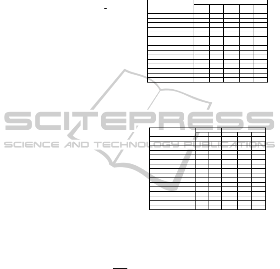
Table 3 shows the results for the different struc-
tural heuristics for the choice of the root. Recall this
choice induces an order σ on the nodes and the row
BE corresponds to the order induced by BE. We re-
mark that the best orders (for the hardest problems of
the test) are the one returned by BE and SC.
Table 3: Comparing different structural orders.
Problems Order
BE LC SC LNS LS
series− 6 − ext 0,09 0,07 0,43 0,07 0,12
series− 7 − ext 0,08 3,48 3,18 3,5 0,96
domino− 100− 100− ext 0,125 0,14 0,49 0,13 0,22
domino− 100− 200− ext 0,24 0,23 0,27 0,23 0,28
domino− 100− 300− ext 0,35 0,36 0,69 0,34 0,51
Langf ord 0,03 0,31 0,91 8,73 1,02
geom− 30a − 4− ext 0,03 0,03 5 0,23 1,02
pigeons− 7 − ext 4,34 4,19 3,5 12 4,23
haystacks − 06− ext 3,33 3,35 3,33 3,22 3,21
Renault1 3,38 3,02 4,41 3,03 3,31
Renault2 8,87 9,02 8,88 / /
Renault − Modified −6 32,07 / 36,09 / /
Renault − Modified −24 21,25 / 18,32 / /
Renault − Modified −30 24,28 / 22,05 / /
Renault − Modified −33 25,42 / 26,01 / /
Renault − Modified −47 19,64 / 21,02 / /
Table 4 shows the results for the different semantic
heuristics for the choice of the root. We remark that
the better choice is given by the MCN heuristic.
Table 4: Comparing different semantic orders.
Problems Size Orders
|V| |E| MCN LCS HN
series− 6 − ext 11 30 0,10 0,38 0,43
series− 7 − ext 12 41 0,55 3,48 0,13
domino− 100− 100− ext 100 100 0,12 0,70 0,49
domino− 100− 200− ext 100 100 0,23 2,32 0,76
domino− 100− 300− ext 100 100 0,36 5,14 0,75
Langf ord 8 32 0,14 0,36 0,09
geom− 30a − 4− ext 30 81 7 1,23 0,03
pigeons− 7 − ext 7 21 11 4,23 4,2
haystacks − 06
−
xt 36 96 6,96 3,32 3,31
Renault1 101 134 3,03 3,02 3,04
Renault2 101 113 7,90 8,36 8,34
Renault −Modi fied − 6 111 147 22,07 / /
Renault −Modi fied − 24 111 159 19,04 / /
Renault −Modi fied − 30 111 154 28,02 / /
Renault −Modi fied − 33 111 154 27,03 / /
Renault −Modi fied − 47 108 149 12,02 / /
Finally, we combine the best structural heuristic
with the best semantic one resulting in BE with MCN
hybrid heuristic. The results are given in Table 5
showing that execution times are always better with
an hybridation of heuristics.
5.5 Heuristics for Choosing Son Nodes
In this section, we experiment different heuristics to
choose the best successor node (function Succ of Al-
gorithm 2) to be solved from the sons of the current
node. We suppose here the root has been already cho-
sen and heuristics have only the choice for the first
son, and it may be considered statically or dynami-
cally.
• Static Choice: the first son to be chosen is the
one with the largest hypertree-width.
• Dynamic Choice: since the best strategy from the
static viewpoint is the one with the minimum of
number of tuples in its relations, we evaluate here
the impact of choosing the next son with the min-
imum number of tuples dynamically. Thus to be
SOLVING NON BINARY CONSTRAINT SATISFACTION PROBLEMS WITH DUAL BACKTRACKING ON
HYPERTREE DECOMPOSITION
153
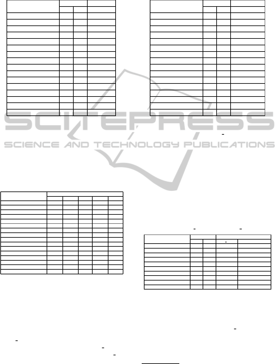
Table 5: Combining structural and semantic heuristics.
Problems Size Method
|V| |E| BE & MCN
series − 6− ext 11 30 0,07
series − 7− ext 12 41 0,06
domino− 100− 100− ext 100 100 0,10
domino− 100− 200− ext 100 100 0,20
domino− 100− 300− ext 100 100 0,30
Langford 8 32 0,04
geom− 30a− 4− ext 30 81 0,04
pigeons− 7− ext 7 21 3,34
haystacks − 06− ext 36 96 2,59
Renault1 101 134 3,38
Renault2 101 113 8,87
Renault − Modified −6 111 147 22,07
Renault − Modified −24 111 159 15,2
Renault − Modified −30 111 154 18,28
Renault − Modified −33 111 154 19,42
Renault − Modified −47 108 149 16,64
consistent with this general strategy we adopt the
same heuristic for choosing the root.
Table 6 gives the results obtained with a static
choice of the successor node and Table 7 gives the
results obtained with a dynamic choice. We observe
here that dynamic choice are better thant the static
one.
Table 6: Static choice of the sons.
Problems Time(s)
BE LC SC LNS LS
series− 6 − ext 0,09 0,07 0,06 0,07 1,01
series− 7 − ext 0,10 12,48 3,18 11,50 9,80
domino− 100− 100− ext 0,12 0,14 0,49 0,132 0,09
domino− 100− 200− ext 0,24 0,23 0,27 0,23 0,27
domino− 100− 300− ext 0,35 0,36 0,69 0,34 0,34
haystacks6 3,33 3,35 4,01 3,22 3,29
Langf ord2 − 4 0,03 0,51 0,05 9,73 1,02
geom− 30a − 4− ext 0,03 0,125 5 0,15 0,19
pigeons− 7 − ext 2,54 4,46 3,5 9,71 5,22
Renault1 3,26 3,63 3,35 3,25 3,32
Renault2 8,71 20 9,25 7,39 > 30
Renault − Modified −6 21 18,07 / / /
Renault − Modified −24 17,09 15,2 / / /
Renault − Modified −30 22,11 28,02 / / /
Renault − Modified −33 24,12 27,03 / / /
Renault − Modified −47 13,01 12,02 / / /
5.6 Comparing with the BTD
Algorithm (J
´
egou et al., 2009)
This section compares our results with the one ob-
tained by BTD for some benchmarks of the Modi-
fied Renault family in Table 8. Due to the fact that
two different machines are used to experiment BTD
and HD DBT (PC Pentium IV 3,4 Ghz for BTD, lap-
top HP Compact 6720 s, 1,7 Ghz for HD DBT) the
reported computational times in the row HD DBT
are normalized according to two benchmarks (Spe, ;
GeB, ). According to these benchmarks, the pentium
IV is 4,5 times faster than the HP Compact 6720s.
Table 7: Dynamic choice of the sons.
Problems Size Method
|V| |E| Dynamic MCN
series − 6− ext 11 30 0,1
series − 7− ext 12 41 0,86
domino− 100− 100− ext 100 100 0,10
domino− 100− 200− ext 100 100 0,20
domino− 100− 300− ext 100 100 0,30
Langford 8 32 0,9
geom− 30a− 4− ext 30 81 1,04
pigeons− 7− ext 7 21 4,34
haystacks − 06− ext 36 96 3,59
Renault1 101 134 3,38
Renault2 101 113 8,87
Renault − Modified −6 111 147 13,07
Renault − Modified −24 111 159 13,2
Renault − Modified −30 111 154 17,28
Renault − Modified −33 111 154 15,42
Renault − Modified −47 108 149 14,64
The reported results for BTD are the best ones found
in (J´egou et al., 2009) and HD DBT present nearly
comparable results. But we have to mention this last
test is not very significative since the detailed imple-
mentation of our approach could be much improved
by using more adequate data structures and general
implementation optimization techniques such the one
used in BTD which is more mature. Notice that the
enumerative algorithms to solve CSP suffer to solve
the modified renault family of benchmarks
2
because
these problems are much structured. Notice that the
symbol / in the table 8 means that we have no result
for the considered instance in (J´egou et al., 2009).
Table 8: BTD HMIN(HD) vs. HD DBT.
Problems Size Time(s)
|V| |E| HD DBT BTD HMIN(HD)
Renault − Modified −4 111 147 16 /
Renault − Modified −6 111 147 4,5 2,70
Renault − Modified −9 111 147 10 /
Renault − Modified −13 111 149 13 /
Renault − Modified −17 111 149 22 3.41
Renault − Modified −24 111 159 3, 7 7,67
Renault − Modified −30 111 154 7, 2 8,25
Renault − Modified −33 111 154 6, 5 /
Renault − Modified −42 108 149 7 2,50
Renault − Modified −47 108 149 3 80,25
6 CONCLUSIONS
In this paper we have presented HD DBT a new al-
gorithm exploiting Hypertree Decomposition to solve
non-binary Constraint Satisfaction Problems. This
algorithm clearly improves the first and basic Algo-
rithm 1 due to Gottlob et al. (Gottlob et al., 2001).
2
http://www.cril.univ-artois.fr/lecoutre/research/
benchmarks
ICAART 2011 - 3rd International Conference on Agents and Artificial Intelligence
154

This last one suffers from the memory explosion
problem and it is consequently inefficient face to large
instances of CSP. Even if HD DBT improves the ba-
sic approach, it is also limited to small structured in-
stances. To improve HD DBT we propose its For-
ward Checking version (HD DBT+FC) which clearly
improves the previous one as FC does for BT. More-
over we proposed and compared several strategies to
achieve the best depth-first traversal of the Hypertree
Decomposition. These strategies concern the choice
of the root, that is the first node and the order between
the sons of a given node to be visited by the algorithm.
The experimental results show that:
• the best choice of the root corresponds to the hard-
est node, meaning the node which mimizes the ra-
tio between the number of solutions and the max-
imal number of solutions;
• the best way to visit the sons of a given node cor-
responds to the dynamic heuristic based on the re-
maining tuples in their associated relations;
• combining the best heuristic for choosing the root
with a dynamic heuristic for choosing the next son
of a given node leads to appreciable results.
Finally we compare our approach with the BTD algo-
rithm (J´egou et al., 2009). From a theoretical point
of view the two approaches are similar in the sense
they are both enumerative algorithms exploiting some
structural decomposition. Our approach differs by
exploring in a dual manner an hypertree decompo-
sition instead of a tree decomposition. We compare
our HD DBT with the best BTD version on different
benchmarks showing HD DBT and BTD have com-
parable performance. To conclude notice that our ap-
proach can gained over with several improved data
structures and different technical optimizations that
we have not yet implemented.
As main perspectives, it would be interesting to ap-
ply HD DBT approach to other structural decompo-
sition methods and to improve the structural decom-
position by taking into account semantic properties of
the CSPs.
REFERENCES
GeekBench benchmarks. http://www.primatelabs.ca/
geekbenchs.
Standard Performance evaluation Corporation (SPEC).
http://www.spec.org.
David Cohen, Peter Jeavons, M. G. (2005). A unified the-
ory of structural tractability for constraint satisfaction
problems. In Proceedings of IJCAI ’ 05.
Dechter, R. (1999). unifying framework for reasoning. Ar-
tificial Intelligence, 113.
Dechter, R. (2003). Constraint Processing. Morgan Kauf-
mann.
Dechter, R. and Pearl, J. (1989). Tree clustering for con-
straint networks. Artificial Intelligence, 38:353–366.
Dermaku, A., Ganzow, T., Gottlob, G., McMahan, B., Mus-
liu, N., and Samer, M. (2005). Heuristic methods for
hypertree decompositions. Technical report, DBAI-R.
Freuder, E. C. (1982). A sufficient condition for backtrack-
free search. Journal of the Association for Computing
Machinery, 29:24–32.
Gottlob, G., Crohe, M., and Musliu, N. (2005). Hyper-
tree decomposition: structure, algorithms and applica-
tions. In Proceeding of 31 st International workshop
WG, Metz.
Gottlob, G., Leone, N., and Scarcello, F. (1999). On
tractable queries and constraints. In Proceedings of
DEXA’99.
Gottlob, G., Leone, N., and Scarcello, F. (2000). A compar-
ison of structural csp decomposition methods. Artifi-
cial Intelligence, 124:243–282.
Gottlob, G., Leone, N., and Scarcello, F. (2001). Hypertree
decompositions: A survey. In Proceedings of MFCS
’01, pages 37–57.
Gottlob, G., Leone, N., and Scarcello, F. (2002). Robbers,
marshals and guards : Theoretic and logical character-
izations of hypertree width. Journal of the ACM.
Greco, G. and Scarcello, F. (2010). On the power of
structural decompositions of graph-based representa-
tions of constraint problems. Artificial Intelligence,
174:382–409.
Grohe, M. and Marx, D. (2006). Constraint solving via frac-
tional edge covers. ACM 2006, C-30(2):101–106.
Gyssens, M., Jeavons, P. G., and Cohen, D. A. (1994).
Decomposing constraint satisfaction problems using
database techniques. Artificial Intelligence, 66:57–89.
Harvey, P. and Ghose, A. (2003). Reducing redundancy in
the hypertree decomposition scheme. In Proceeding
of ICTAI’03, pages 548–555, Montreal.
Jeavons, P. G., A, C. D., and Gyssens, M. (1994). A struc-
tural decomposition for hypergraphs. Contemporary
Mathematics, 178:161–177.
J´egou, P., Ndiaye, S. N., and Terrioux, C. (2009). Com-
bined strategies for decomposition-based methods for
solving csps. In Proceedings of the 21st IEEE Interna-
tional Conference on Tools with Artificial Intelligence
(ICTAI 2009), pages 184–192.
J´egou, P. and Terrioux, C. (2003). Hybrid backtrack-
ing bounded by tree-decomposition of constraint net-
works. Artificial Intelligence,, 146:43–75.
Korimort, T. (2003). Heuristic hypertree decomposition.
AURORA TR 2003-18.
Montanari, U. (1974). Networks of constraints: Fundamen-
tal properties and applications to pictures processing.
Information Sciences, 7:95–132.
Musliu, N. and Schafhauser, W. (2005). Genetic algorithms
for generalized hypertree decompositions. European
Journal of Industrial Engineering, 1(3):317–340.
SOLVING NON BINARY CONSTRAINT SATISFACTION PROBLEMS WITH DUAL BACKTRACKING ON
HYPERTREE DECOMPOSITION
155

Pang, W. and Goodwin, S. D. (1997). Constraint-directed
backtracking. In 1Oth Australian Joint Conference on
AI, pages 47–56, Perth, Western Australia.
Pang, W. and Goodwin, S. D. (2003). A graph based back-
tracking algorithm for solving general csps. In Lec-
ture Notes in Computer Sciences of AI 2003, pages
114–128, Halifax.
Samer, M. (2005). Hypertree-decomposition via branch-
decomposition. In Proceedings of the 19th interna-
tional joint conference on Artificial intelligence, pages
1535–1536, Edinburgh, Scotland.
Sathiamoorthy, S. and Andersen, H. R. (2007). Backtrack-
ing procedures for hypertree, hyperspread and con-
nected hypertree decomposition of csps. In Proceed-
ings of the IJCAI-07.
ICAART 2011 - 3rd International Conference on Agents and Artificial Intelligence
156
