LOCAL FEATURE BASED IMAGE SIMILARITY FUNCTIONS
FOR kNN CLASSIFICATION
Giuseppe Amato and Fabrizio Falchi
Institute of Information Science and Technology, via G. Moruzzi 1, Pisa, Italy
Keywords:
Image classification, Image content recognition, Pattern recognition, Machine learning.
Abstract:
In this paper we consider the problem of image content recognition and we address it by using local features
and kNN based classification strategies. Specifically, we define a number of image similarity functions relying
on local feature similarity and matching with and without geometric constrains. We compare their performance
when used with a kNN classifier. Finally we compare everything with a new kNN based classification strategy
that makes direct use of similarity between local features rather than similarity between entire images.
As expected, the use of geometric information offers an improvement over the use of pure image similarity.
However, surprisingly, the kNN classifier that use local feature similarity has a better performance than the
others, even without the use of geometric information.
We perform our experiments solving the task of recognizing landmarks in photos.
1 INTRODUCTION
Image content recognition is a very important issue
that is being studied by many scientists worldwide.
In fact, with the explosion of the digital photography,
during the last decade, the amount of digital pictures
available on-line and off-line has extremely increased.
However, many of these pictures remain unannotated
and are stored with generic names on personal com-
puters and on on-line services. Currently, there are
no tools and effective technologies to help users in
searching for pictures by real content, when they are
not explicitly annotated. Therefore, it is becoming
more and more difficult for users to retrieve even their
own pictures.
A picture contains a lot of implicit conceptual in-
formation that is not yet possible to exploit entirely
and effectively. Automatically content based image
recognition opens up opportunities for new advanced
applications. For instance, pictures themselves might
be used as queries on the web. An example in this
direction is the service “Google Goggles” (Google,
2010) recently launched by Google, that allows you
to obtain information about a monument through your
smartphone using this paradigm.
Note that, even if many smartphones and cameras
are equipped with a GPS and a compass, the geo-
reference obtained with this is not enough to infer
what the user is actually aiming at. Content analy-
sis of the picture is still needed to determine more
precisely the user query or the annotation to be as-
sociated with a picture.
A promising approach toward image content
recognition is the use of classification techniques to
associate images with classes (labels) according to
their content. For instance, if an image contains a car,
it might be automatically associated with the class car
(labelled with the label car).
In this paper we study the problem of image con-
tent recognition by using SIFT (Lowe, 2004) and
SURF (Bay et al., 2006) local features, to represent
image visual content, and kNN based classifiers to de-
cide about the presence of conceptual content.
In more details we will define 20 different func-
tions that measure similarity between images. These
functions are defined using various options and com-
binations of local feature matching and similarities.
Some of them also take into consideration geometric
properties of the matching local features. These func-
tions are used in combination of a standard Single-
label Distance-Weighted kNN algorithm. In addition
we also propose a new classification algorithm that
extend the traditional kNN classifiers by making di-
rect use of similarity between local features, rather
than similarity between entire images.
We will see that the similarity functions that also
make use of geometric considerations offer a better
performance than the others. However, the new kNN
157
Amato G. and Falchi F..
LOCAL FEATURE BASED IMAGE SIMILARITY FUNCTIONS FOR KNN CLASSIFICATION.
DOI: 10.5220/0003185401570166
In Proceedings of the 3rd International Conference on Agents and Artificial Intelligence (ICAART-2011), pages 157-166
ISBN: 978-989-8425-40-9
Copyright
c
 2011 SCITEPRESS (Science and Technology Publications, Lda.)

based classifier that exploit directly the similarity be-
tween local features has an higher performance even
without using geometric information.
The paper is organized as follows. In Section 3
we briefly introduce local features. In Section 4 we
present various iamge similarity features relying on
local features to be used with a kNN classification al-
gorithm. Section 5 propose a novel classification ap-
proach. Finally, Sections 6 and 7 presents the experi-
mental results.
2 RELATED WORK
The first approach to recognizing location from mo-
bile devices using image-based web search was pre-
sented in (Yeh et al., 2004). Two image matching met-
rics were used: energy spectrum and wavelet decom-
positions. Local features were not tested.
In the last few years the problem of recogniz-
ing landmarks have received growing attention by
the research community. In (Serdyukov et al., 2009)
methods for placing photos uploaded to Flickr on the
World map was presented. In the proposed approach
the images were represented by vectors of features of
the tags, and visual keywords derived from a vector
quantization of the SIFT descriptors.
In (Kennedy and Naaman, 2008) a combination of
context- and content-based tools were used to gener-
ate representative sets of images for location-driven
features and landmarks. Visual information is com-
bined with the textual metadata while we are only
considering content-based classification.
In (Zheng et al., 2009), Google presented its ap-
proach to building a web-scale landmark recognition
engine. Most of the work reported was used to im-
plement the Google Goggles service (Google, 2010).
The approach makes use of the SIFT feature. The
recognition is based on best matching image search-
ing, while our novel approach is based on local fea-
tures classification. In (Chen et al., 2009) a survey
on mobile landmark recognition for information re-
trieval is given. Classification methods reported as
previously presented in the literature include SVM,
Adaboost, Bayesian model, HMM, GMM. The kNN
based approach which is the main focus of this paper
is not reported in that survey. In (Fagni et al., 2010),
various MPEG-7 descriptors have been used to build
kNN classifier committees. However local features
were not considered.
In (Boiman et al., 2008) the effectiveness of NN
image classifiers has been proved and an innovative
approach based on Image-to-Class distance that is
similar in spirit to our approach has been proposed.
3 LOCAL FEATURES
The approach described in this paper focuses on the
use of image local features. Specifically, we per-
formed our tests using the SIFT (Lowe, 2004) and
SURF (Bay et al., 2006) local features. In this sec-
tion, we briefly describe both of them.
The Scale Invariant Feature Transformation
(SIFT) (Lowe, 2004) is a representation of the low
level image content that is based on a transformation
of the image data into scale-invariant coordinates rel-
ative to local features. Local feature are low level de-
scriptions of keypoints in an image. Keypoints are
interest points in an image that are invariant to scale
and orientation. Keypoints are selected by choosing
the most stable points from a set of candidate loca-
tion. Each keypoint in an image is associated with
one or more orientations, based on local image gra-
dients. Image matching is performed by comparing
the description of the keypoints in images. For both
detecting keypoints and extracting the SIFT features
we used the public available software developed by
David Lowe
1
.
The basic idea of Speeded Up Robust Features
(SURF) (Bay et al., 2006) is quite similar to SIFT.
SURF detects some keypoints in an image and de-
scribes these keypoints using orientation information.
However, the SURF definition uses a new method for
both detection of keypoints and their description that
is much faster still guaranteeing a performance com-
parable or even better than SIFT. Specifically, key-
point detection relies on a technique based on a ap-
proximation of the Hessian Matrix. The descriptor of
a keypoint is built considering the distortion of Haar-
wavelet responses around the keypoint itself. For
both, detecting keypoints and extracting the SURF
features, we used the public available noncommercial
software developed by the authors
2
.
4 IMAGE SIMILARITY BASED
CLASSIFIER
In this section we discuss how traditional kNN classi-
fication algorithms can be applied to the task of clas-
sifying images described by local features, as for in-
stance SIFT or SURF. In particular, we define 20 im-
age similarity measures based on local features de-
scription. These will be later on compared to the new
classification strategy that we propose in Section 5.
1
http://people.cs.ubc.ca/ lowe/
2
http://www.vision.ee.ethz.ch/ surf
ICAART 2011 - 3rd International Conference on Agents and Artificial Intelligence
158

4.1 Single-label Distance-weighted kNN
Given a set of documents D and a predefined set
of classes (also known as labels, or categories)
C = {c
1
,...,c
m
}, single-label document classification
(SLC) (Dudani, 1975) is the task of automatically ap-
proximating, or estimating, an unknown target func-
tion Φ : D → C, that describes how documents ought
to be classified, by means of a function
ˆ
Φ : D → C,
called the classifier, such that
ˆ
Φ is an approximation
of Φ.
A popular SLC classification technique is the
Single-label distance-weighted kNN. Given a training
set Tr containing various examples for each class c
i
,
it assigns a label to a document in two steps. Given
a document d
x
(an image for example) to be classi-
fied, it first executes a kNN search between the ob-
jects of the training set. The result of such operation
is a list χ
k
(d
x
) of labelled documents d
i
belonging to
the training set ordered with respect to the decreas-
ing values of the similarity s(d
x
,d
i
) between d
x
and
d
i
. The label assigned to the document d
x
by the clas-
sifier is the class c
j
∈ C that maximizes the sum of the
similarity between d
x
and the documents d
i
, labelled
c
j
, in the kNN results list χ
k
(d
x
)
Therefore, first a score z(d
x
,c
i
) for each label is
computed for any label c
i
∈ C:
z(d
x
,c
j
) =
∑
d
i
∈χ
k
(d
x
) : Φ(d
i
)=c
j
s(d
x
,d
i
) .
Then, the class that obtains the maximum score is
chosen:
ˆ
Φ
s
(d
x
) = argmax
c
j
∈C
z(d
x
,c
j
) .
It is also convenient to express a degree of confi-
dence on the answer of the classifier. For the Single-
label distance-weighted kNN classifier described here
we defined the confidence as 1 minus the ratio be-
tween the score obtained by the second-best label and
the best label, i.e,
ν
doc
(
ˆ
Φ
s
,d
x
) = 1 −
arg max
c
j
∈C−
ˆ
Φ
s
(d
x
)
z(d
x
,c
j
)
argmax
c
j
∈C
z(d
x
,c
j
)
.
This classification confidence can be used to de-
cide whether or not the predicted label has an high
probability to be correct.
4.2 Image Similarity
In order the kNN search step to be executed, a sim-
ilarity function between images should be defined.
Global features, generally, are defined along with a
similarity (or a distance) function. Therefore, simi-
larity between images, is computed as the similarity
between the corresponding global features. On the
other hand, a single image has several local features.
Therefore, computing the similarity between two im-
ages requires combining somehow the similarities be-
tween their numerous local features.
In the following we define a function for comput-
ing similarity between images on the basis of their lo-
cal features that is derived from the work presented
in (Lowe, 2004). In the experiments, at the end
of this paper, we will compare the performance of
the similarity function, when used with the single-
label distance-weighted kNN classification technique,
against the local feature based classification algorithm
proposed in Section 5.
4.2.1 Local Feature Similarity
The Computer Vision literature related to local fea-
tures, generally uses the notion of distance, rather
than that of similarity. However in most cases a sim-
ilarity function s() can be easily derived from a dis-
tance function d(). For both SIFT and SURF the Eu-
clidean distance is typically used as measure of dis-
similarity between two features (Lowe, 2004; Bay
et al., 2006).
Let d(p
1
, p
2
) ∈ [0, 1] be the normalized distance
between two local features p
1
and p
2
. We can define
the similarity as:
s(p
1
, p
2
) = 1 − d(p
1
, p
2
)
Obviously 0 ≤ s(p
1
, p
2
) ≤ 1 for any p
1
and p
2
.
4.2.2 Local Features Matching
A useful aspect that is often used when dealing with
local features is the concept of local feature matching.
In (Lowe, 2004), a distance ratio matching scheme
was proposed that has also been adopted by (Bay
et al., 2006) and many others. Let’s consider a lo-
cal feature p
x
belonging to an image d
x
(i.e. p
x
∈ d
x
)
and an image d
y
. First, the point p
y
∈ d
y
closest to p
x
(in the remainder NN
1
(p
x
,d
y
)) is selected as candi-
date match. Then, the distance ratio σ(p
x
,d
y
) ∈ [0,1]
of closest to second-closest neighbors of p
x
in d
y
is
considered. The distance ratio is defined as:
σ(p
x
,d
y
) =
d(p
x
,NN
2
(p
x
,d
y
))
d(p
x
,NN
1
(p
x
,d
y
))
Finally, p
x
and NN
1
(p
x
,d
y
) are considered match-
ing if the distance ratio σ(p
x
,d
y
) is smaller than a
given threshold. Thus, a function of matching be-
tween p
x
∈ d
x
and an image d
y
is defined as:
m(p
x
,d
y
) =

1 if σ(p
x
,d
y
) < c
0 otherwise
LOCAL FEATURE BASED IMAGE SIMILARITY FUNCTIONS FOR kNN CLASSIFICATION
159

In (Lowe, 2004), c = 0.8 was proposed reporting that
this threshold allows to eliminate 90% of the false
matches while discarding less than 5% of the cor-
rect matches. In Section 7 we report an experimen-
tal evaluation of classification effectiveness varying c
that confirms the results obtained by Lowe. Please
note, that this parameter will be used in defining the
image similarity measure used as a baseline and in
one of our proposed local feature based classifiers.
For Computer Vision applications, the distance ra-
tio described above is used for selecting good candi-
date matches. More sophisticated algorithms are then
used to select actual matches from the selected ones
considering geometric information as scale, orienta-
tion and coordinates of the interest points. In most of
the cases a Hough transform (Ballard, 1981) is used
to search for keys that agree upon a particular model
pose. To avoid the problem of boundary effects in
hashing, each match is hashed into the 2 closest bins
giving a total of 16 entries for each hypothesis in the
hash table. This method has been proposed for SIFT
(Lowe, 2004) and is very similar to the weak geome-
try consistency check used in (J
´
egou et al., 2010).
Thus, we define the set M
h
(d
x
,d
y
) as the matching
points in the most populated entry in the Hash table
containing the Hough transform of the matches in d
y
obtained using the distance ratio criteria.
4.3 Similarity Measures
In this section, we define 5 different image similarity
measures approaches and 4 different versions of each
of them for a total of 20 measures.
4.3.1 1-NN Similarity Average – s
1
The simplest similarity measure only consider the
closest neighbor for each p
x
∈ d
x
and its distance from
the query point p
x
. The similarity between two docu-
ments d
x
and d
y
can be defined as the average similar-
ity between the local features in d
x
and their closest
neighbors in d
y
. Thus, we define the 1-NN Similarity
Average as:
s
1
(d
x
,d
y
) =
1
|
d
x
|
∑
p
x
∈d
x
max
p
y
∈d
y
(s(p
x
, p
y
))
For simplicity, we indicate the number of local
features in an image d
x
as
|
d
x
|
.
4.3.2 Percentage of Matches – s
m
A reasonable measure of similarity between two im-
age d
x
and d
y
is the percentage of local features in d
x
that have a match in d
y
. Using the distance ratio crite-
rion described in 4.2.2 for individuating matches, we
define the Percentage of Matches similarity function
s
m
as follows:
s
m
(d
x
,d
y
) =
1
|
d
x
|
∑
p
x
∈d
x
m(p
x
,d
y
)
where m(p
x
,d
y
) is 1 if p
x
has a match in d
y
and 0
otherwise as defined in Section 4.2.2.
4.3.3 Distance Ratio Average – s
σ
The matching function m(p
x
,d
y
) used in the Percent-
age of Matches similarity function is based on the ra-
tio between closest to second-closest neighbors for fil-
tering candidate matches as proposed in (Lowe, 2004)
and reported in Section 4.2.2. However, this distance
ratio value can be used directly to define a Distance
Ratio Average function between two images d
x
and d
y
as follows:
s
σ
(d
x
,d
y
) =
1
|
d
x
|
∑
p
x
∈d
x
σ(p
x
,d
y
)
Please note that function does not require a dis-
tance ratio c threshold to be set.
4.3.4 Hough Transform Matches Percentage – s
h
As mentioned in Section 4.2.2, an Hough transform is
often used to search for keys that agree upon a partic-
ular model pose. The Hough transform can be used to
define a Hough Transform Matches Percentage:
s
h
(d
x
,d
y
) =
|M
h
(d
x
,d
y
)|
|
d
x
|
where M
h
(d
x
,d
y
) is the subset of matches voting
for the most voted pose. For the experiments, we used
the same parameters proposed in (Lowe, 2004), i.e.
bin size of 30 degrees for orientation, a factor of 2 for
scale, and 0.25 times the maximum model dimension
for location.
4.3.5 Managing the Asymmetry
All the proposed similarity functions are not symmet-
ric, i.e., s(d
x
,d
y
) = s(d
y
,d
x
) does not hold. Consider
the case in which the set of local features belonging
to d
x
is a subset of the ones belonging to d
y
. In this
case the similarity s(d
x
,d
y
) is 1 while the same does
not hold for s(d
y
,d
x
).
In searching for images similar to d
x
, it is not
clear in advance whether s(d
x
,d
y
) or s(d
y
,d
x
) would
be a better similarity measure for the recognition task.
Thus, we tested various combinations.
Given an image d
Te
belonging to Te (i.e., an image
that we want to automatically classify), and an image
ICAART 2011 - 3rd International Conference on Agents and Artificial Intelligence
160

d
Tr
belonging to Tr (i.e., an image for which the class
label is known in advance) we define various versions
of the similarities defined before:
• s
Te
(d
Te
,d
Tr
) = s(d
Te
,d
Tr
) is the canonical ap-
proach which tries to find points in the test image
that are similar to the ones in the training one.
• s
Tr
(d
Te
,d
Tr
) = s(d
Tr
,d
Te
) is the inverse approach
which uses the points in training documents as
queries.
• s
or
(d
Te
,d
Tr
) = max(s(d
Te
,d
Tr
),s(d
Tr
,d
Te
)) is the
fuzzy or of s
Te
and s
Tr
. This considers equivalent
two images if any of the two is a crop of the other.
• s
and
(d
Te
,d
Tr
) = min(s(d
Te
,d
Tr
),s(d
Tr
,d
Te
)) is
the fuzzy and of s
Te
and s
Tr
. This never considers
equivalent two images if any of the two is a crop
of the other.
• s
avg
(d
Te
,d
Tr
) = (s(d
Te
,d
Tr
)+s(d
Tr
,d
Te
))/2 is the
mean of s
Te
and s
Tr
.
Thus, we have defined 5 versions of our 4 similar-
ity measures for a total of 20 similarity measures that
will be denoted as s
m,Te
,s
m,Tr
,s
m,or
,...,s
h,Te
, etc.
5 LOCAL FEATURE BASED
IMAGE CLASSIFIER
In the previous section, we considered the classifica-
tion of an image d
x
as a process of retrieving the most
similar ones in the training set Tr and then applying
a kNN classification technique in order to predict the
class of d
x
.
In this section, we propose a new approach that
first assigns a label to each local feature of an image.
The label of the image is then assigned by analyzing
the labels and confidences of its local features.
This approach has the advantage that any access
method for similarity search in metric spaces (Zezula
et al., 2006) can be used to speed-up classification.
The proposed Local Feature Based Image Classi-
fiers classify an image d
x
in two steps:
1. First each local feature p
x
belonging to d
x
is clas-
sified considering the local features of the images
in Tr;
2. Second the whole image is classified considering
the class assigned to each local feature and the
confidence of the classification.
Note that classifying individually the local fea-
tures, before assigning the label to an image, we
might loose the implicit dependency between interest
points of an image. However, surprisingly, we will
see that this method offers better effectiveness than
the baseline approach. In other words we are able to
improve at the same time both efficiency and effec-
tiveness.
In the following, we assume that the label of each
local feature p
x
, belonging to images in the training
set Tr, is the label assigned to the image it belongs to
(i.e., d
x
). Following the notation used in Section 4,
∀p
x
∈ d
x
, ∀d
x
∈ Tr , Φ(p
x
) = Φ(d
x
).
In other words, we assume that the local features
generated over interest points of the images in the
training set can be labeled as the image they belong
to. Note that the noise introduced by this label propa-
gation from the whole image to the local features can
be managed by the local features classifier. In fact,
we will see that when very similar training local fea-
tures are assigned to different classes, a local feature
close to them is classified with a low confidence. The
experimental results reported in Section 7 confirm the
validity of this assumption.
As we said before, given p
x
∈ d
x
, a classifier
ˆ
Φ re-
turns both a class
ˆ
Φ(p
x
) = c
i
∈ C to which it believes
p
x
to belong and a numerical value ν(
ˆ
Φ, p
x
) that rep-
resents the confidence that
ˆ
Φ has in its decision. High
values of ν correspond to high confidence.
5.1 Local Feature Classifier
Among all the possible approach for assigning a label
to a interest point, the simplest is to consider the label
of its closest neighbor in Tr. The confidence value
can be evaluated using the idea of the distance ratio
discussed in Section 4.2.2.
We thus define a local feature based classifier
ˆ
Φ
m
(p
x
) that assign a candidate label
ˆ
Φ
m
(p
x
) as the
one of the nearest neighbor in Tr closest to p
x
(i.e.,
NN
1
(p
x
,Tr)):
ˆ
Φ
m
(p
x
) = Φ(NN
1
(p
x
,Tr))
The confidence here plays the role of a matching
function, where the idea of the distance ratio is used
to decide if the candidate label is a good match:
ν(
ˆ
Φ
m
, p
x
) =

1 if
˙
σ(p
x
,t
r
) < c
0 otherwise
The distance ratio
˙
σ here is computed consider-
ing the nearest local feature to p
x
and the closest local
feature that has a label different than the nearest lo-
cal feature. This idea follows the suggestion given
by Lowe in (Lowe, 2004), that whenever there are
multiple training images of the same object, then the
second-closest neighbor to consider for the distance
ratio evaluation should be the closest neighbor that is
known to come from a different object than the first.
LOCAL FEATURE BASED IMAGE SIMILARITY FUNCTIONS FOR kNN CLASSIFICATION
161

Following this intuition, we define the similarity ratio
˙
σ as:
˙
σ(p
x
,T
r
) =
d(p
x
,NN
∗
2
(p
x
,Tr))
d(p
x
,NN
1
(p
x
,Tr))
where NN
∗
2
(p
x
,Tr) is the closest neighbor that is
known to be labeled differently than the first as sug-
gested in (Lowe, 2004).
The parameter c used in the definition of the con-
fidence is the equivalent of the one used in (Lowe,
2004) and (Bay et al., 2006). We will see in Section
7 that c = 0.8 proposed in (Lowe, 2004) by Lowe is
able to guarantee good effectiveness. It is worth to
note that c is the only parameter to be set for this clas-
sifier considering that the similarity search performed
over the local features in Tr does not require a param-
eter k to be set.
5.2 Whole Image Classification
As we said before, the local feature based feature clas-
sification is composed of two steps (see Section 5). In
previous section we have dealt with the issue of clas-
sifying the local feature of an image. Now, in this
section, we discuss the second phase of the local fea-
ture based classification of images. In particular we
consider the classification of the whole image given
the label
ˆ
Φ(p
x
) and the confidence ν(
ˆ
Φ, p
x
) assigned
to its local features p
x
∈ d
x
during the first phase.
To this aim, we use a confidence-rated majority
vote approach. We first compute a score z(p
x
,c
i
) for
each label c
i
∈ C. The score is the sum of the confi-
dence obtained for the local features predicted as c
i
.
Formally,
z(d
x
,c
i
) =
∑
p
x
∈d
x
,
ˆ
Φ(p
x
)=c
i
ν(
ˆ
Φ, p
x
) .
Then, the label that obtains the maximum score is
chosen:
ˆ
Φ(d
x
) = argmax
c
j
∈C
z(d
x
,c
j
) .
As measure of confidence for the classification of
the whole image we use ratio between the predicted
and the second best class:
ν
img
(
ˆ
Φ,d
x
) = 1 −
arg max
c
j
∈C−
ˆ
Φ(p
x
)
z(d
x
,c
j
)
argmax
c
i
∈C
z(d
x
,c
i
)
.
This whole image classification confidence can be
used to decide whether or not the predicted label has
an high probability to be correct. In the experimen-
tal results Section 7 we will show that the proposed
confidence is reasonable.
6 EVALUATION SETTINGS
For evaluating the various classifiers we need at least:
a data set, an interest points detector, a local feature
extractor, some performance measures. In the follow-
ing, we present all the evaluation setting we used for
the experimentation.
Figure 1: Example images taken from the dataset.
6.1 The Dataset
The dataset that we used for our tests is composed of
1,227 photos of landmarks located in Pisa and was
used also in (Amato et al., 2010). The photos have
been crawled from Flickr, the well known on-line
photo service. The dataset we built is publicly avail-
able. The IDs of the photos used for these experi-
ments together with the assigned label and extracted
features can be downloaded from (Falchi, 2010). In
the following we list the classes that we used and the
number of photos belonging to each class. In Figure
1 we reported an example for each class in the same
order as they are reported in the list below:
• Leaning Tower (119 photos) – leaning campanile
• Duomo (130 photos) – the cathedral of St. Mary
• Battistero (104 photos) – the baptistery of St. John
• Camposanto Monumentale (exterior) (46 photos)
• Camposanto Monumentale (field) (113 photos)
• Camposanto Monumentale (portico) (138 photos)
• Chiesa della Spina (112 photos) – Gothic church
• Palazzo della Carovana (101 photos) – building
• Palazzo dell’Orologio (92 photos) – building
• Guelph tower (71 photos)
• Basilica of San Piero (48 photos) – church
• Certosa (53 photos) – charter house
In order to build and evaluating a classifier for
these classes, we divided the dataset in a training set
(Tr) consisting of 226 photos (approximately 20% of
ICAART 2011 - 3rd International Conference on Agents and Artificial Intelligence
162

the dataset) and a test set (Te) consisting of 921 (ap-
proximately 80% of the dataset). The image resolu-
tion used for feature extraction is the standard resolu-
tion used by Flickr i.e., maximum between width and
height equal to 500 pixels.
The total number of local features extracted by the
SIFT and SURF detectors were about 1,000,000 and
500,000 respectively.
6.2 Performance Measures
For evaluating the effectiveness of the classifiers in
classifying the documents of the test set we use
the micro-averaged accuracy and micro- and macro-
averaged precision, recall and F
1
.
Micro-averaged values are calculated by con-
structing a global contingency table and then calcu-
lating the measures using these sums. In contrast
macro-averaged scores are calculated by first calcu-
lating each measure for each category and then taking
the average of these. In most of the cases we reported
the micro-averaged values for each measure.
Precision is defined as the ratio between correctly
predicted and the overall predicted documents for a
specific class. Recall is the ratio between correctly
predicted and the overall actual documents for a spe-
cific class. F
1
is the harmonic mean of precision and
recall.
Note that for the single-label classification task,
micro-averaged accuracy is defined as the number
of documents correctly classified divided by the total
number of documents in the test set and it is equiv-
alent to the micro-averaged precision, recall and F
1
scores.
7 EXPERIMENTAL RESULTS
In this section we report the experimental results ob-
tained for all the 20 image similarity based and lo-
cal feature based classifiers. For the image similarity
based classifier results are reported for each similarity
measure defined in Section 4.3. We also show that the
proposed measure of confidence can be used to im-
prove effectiveness on classified images accepting a
small percentage of not classified objects.
7.1 Image Similarity based Classifiers
In Table 1, Accuracy and macro averaged F
1
of the
image similarity based classifiers for the 20 similarity
functions defined in Section 4 are reported. Note that
the single-label distance-weighted kNN technique has
a parameter k that determines the number of closest
neighbors retrieved in order to classify a given image
(see Section 4). This parameter should be set dur-
ing the training phase and is kept fixed during the test
phase. However, in our experiments we decided to re-
port the result obtained ranging k between 1 and 100.
For simplicity, in Table 1, we report the best perfor-
mance obtained and the k for which it was obtained.
Moreover, we report the performance obtained for
k = 1 which is a particular case in which the kNN
classifier simply consider the closest image.
Let’s first consider the approach used for manag-
ing the asymmetry of the distance functions discussed
in Section 4.3.5. The best approach for all the simi-
larity functions using both SIFT and SURF features
is the fuzzy and, i.e., s
*,and
. The more traditional ap-
proach s
*,Te
is the second best in most of the cases.
On the contrary, s
*,Tr
always offers the worst perfor-
mance. In other words, the best results were obtained
when the similarity between two images is computed
as the minimum of the similarity obtained consider-
ing as query in turn the test image local features and
the training images. The result is the same both when
using SIFT and SURF.
The Hough Transform Matches Percentage (s
h
)
similarity function is the best choice for both SIFT
and SURF for all the 5 versions for managing the
asymmetry. The geometric information considered by
this function allows to obtain significantly better per-
formance in particular for SURF.
The second best is Distance Ratio Average (s
σ
)
which only considers the distance ratio as match-
ing criterion. Please note that s
σ
does not require a
distance ratio threshold (c) because it weights every
match considering the distance ratio value. Moreover,
s
σ
performs sightly better than Percentage of Matches
(s
m
) which requires the threshold c to be set.
The results obtained by the 1-NN Similarity Aver-
age (s
1
) function show that considering just the dis-
tance between a local features and its closest neigh-
bors gives worst performance than considering the
similarity ratio s
σ
. In other words, the similarity be-
tween a local feature and its closest neighbor is mean-
ingful only if compared to the other nearest neighbors,
which is exactly what the distance ratio does.
Regarding the parameter k it is interesting to note
that the k value for which the best performance was
obtained for each similarity measure is typically much
higher for SURF than SIFT. In other words, the test
image closest neighbors in the training set are more
relevant using SIFT than using SURF.
This is more evident in Figure 2 where we report
the accuracy obtained for k between 1 and 100 by
both SIFT and SURF using the s
m,Te
similarity func-
tion. SIFT obtains the best performance for smaller
LOCAL FEATURE BASED IMAGE SIMILARITY FUNCTIONS FOR kNN CLASSIFICATION
163

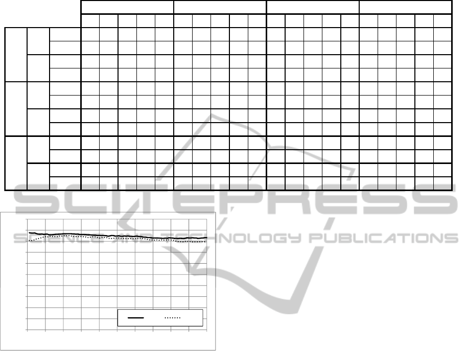
Table 1: Image similarity based classifier (
ˆ
Φ
s
) performance obtained using various image similarity functions.
Te Tr or and avg Te Tr or and avg Te Tr or and avg Te Tr or and avg
SIFT
.75 .52 .55 .85 .82 .88 .80 .81 .90 .88 .89 .80 .81 .91 .89 .92 .88 .88
.93
.91
SURF
.79 .70 .73 .80 .82 .85 .73 .76 .88 .86 .82 .73 .75 .87 .84 .89 .76 .79
.92
.86
SIFT
.72 .55 .56 .84 .84 .86 .80 .80 .89 .86 .87 .80 .81 .91 .88 .90 .87 .86
.93
.90
SURF
.76 .67 .70 .78 .80 .83 .70 .74 .87 .84 .81 .68 .73 .86 .82 .87 .74 .77
.89
.85
SIFT
.73 .52 .55 .85 .82 .88 .78 .80 .90 .88 .89 .78 .80 .91 .88 .91 .87 .87
.93
.91
SURF
.79 .63 .67 .80 .82 .81 .60 .62 .86 .79 .81 .63 .64 .84 .76 .87 .66 .68
.90
.81
SIFT
.72 .55 .53 .84 .84 .86 .78 .80 .89 .86 .87 .79 .80 .90 .87 .90 .86 .86
.92
.90
SURF
.76 .63 .67 .78 .80 .79 .65 .65 .84 .78 .80 .67 .67 .83 .77 .85 .68 .70
.89
.81
SIFT
9 1 1 1 1 1 7 4 2 3 1 5 5 3 5 2 3 9 2 1
SURF
3 6 8 1 1 20 28 42 14 20 8 23 17 11 14 21 35 39 11 18
SIFT
1 1 1 1 1 1 7 4 3 3 1 5 5 3 5 2 8 5 9 9
SURF
1 6 3 1 1 18 28 19 23 20 8 5 17 11 14 21 14 30 3 28
Best
k
Acc
F
1
Acc
F
1
Best
k =1
F
1
s
m
- Perc. of Matches s
σ
- Avg Sim. Ratio s
1
- Avg 1-NN
similarity function
Acc
s
h
- Hough Transform
version
0.4
0.5
0.6
0.7
0.8
0.9
1.0
Accuracy
0.0
0.1
0.2
0.3
0.4
0.5
0.6
0.7
0.8
0.9
1.0
0 10 20 30 40 50 60 70 80 90 100
Accuracy
k
SIFT
SURF
Figure 2: Accuracy obtained for various k using the s
m,Te
similarity function by both SIFT and SURF.
values of k with respect to SURF. Moreover, SIFT
performance is generally higher than SURF.
It is interesting to note that performance obtained
for k = 1 is typically just slightly worst than that of
the best k. Thus, k = 1 gives very good performance
even if a better k could be selected during a learning
phase.
Two of the similarity measures proposed in Sec-
tion 4.3 require a parameter to be set. In particular,
the similarity measures Percentage of Matches (s
m
)
and Hough Transform Matches Percentage (s
h
) use
the matching function defined in Section 4.2.2 that re-
quires a threshold for the distance ratio threshold (c)
to be fixed in advance.
In Figure 3 we report the performance obtained
by using the Percentage of Matches classifier, i.e., the
image similarity based classifier
ˆ
Φ
s
using the similar-
ity measure s
m
. For each distance ratio threshold c we
report the best result obtained for k between 0 and
100. As mentioned in Section 4.2.1, in the paper
where SIFT (Lowe, 2004) was presented, Lowe sug-
gested to use 0.8 as distance ratio threshold (c). The
results confirm that the threshold proposed in (Lowe,
2004) is the best for both SIFT and SURF and that the
algorithm is stable around this values. In Table 1, re-
sults were reported for s
m
and s
h
with c = 0.8 for both
SIFT and SURF.
Let us now consider the confidence ν
doc
assigned
to the predicted label of each image (see Section 4.1).
This confidence can be used to obtain greater accu-
racy at the price of a certain number of false dis-
missals. In fact, a confidence threshold can be used
to filter all the label assigned to an image with a con-
fidence ν
doc
less than the threshold. In Figure 4 we
report the accuracy obtained by the s
h,and
measure us-
ing SIFT, varying the confidence threshold between 0
and 1. We also report the percentage of images in Te
that were not classified together with the percentage
of images that where actually correctly classified but
that were filtered because of the threshold. Note that
for ν
doc
= 0.3 the accuracy of classified objects rise
from 0.93 to 0.99 obtained for ν
doc
= 0. At the same
time the percentage of correctly predicted images that
are filtered (i.e., the classifier does not assign a label
because of the low confidence threshold ν
doc
) is less
than 10%.
This prove that the measure of confidence defined
is meaningful. However, the best confidence thresh-
old to be used depends on the task. Sometimes it
could be better to try to guess the class of an image
even if we are not sure, while in other cases it might
be better to assign a label only if the classification has
an high confidence.
ICAART 2011 - 3rd International Conference on Agents and Artificial Intelligence
164

0.3
0.4
0.5
0.6
0.7
0.8
0.9
1.0
SIFT Accuracy
0.0
0.1
0.2
0.3
0.4
0.5
0.6
0.7
0.8
0.9
1.0
0 0.1 0.2 0.3 0.4 0.5 0.6 0.7 0.8 0.9 1
Threshold c used for local features matching
SIFT Accuracy
SURF Accuracy
SIFT Macro F1
SURF Macro F1
Figure 3: Accuracy and Macro F
1
obtained for various
matching threshold by the image similarity based classifier
(
ˆ
Φ
s
) using the s
m,Tr
similarity measure and SIFT.
0,5
0,6
0,7
0,8
0,9
1
Accuracy on Classified
Not Classified Perc.
Correctly Classified Losts Perc.
0
0,1
0,2
0,3
0,4
0,5
0,6
0,7
0,8
0,9
1
0 0,1 0,2 0,3 0,4 0,5 0,6 0,7 0,8 0,9 1
Image classification confidence threshold
ν
νν
ν
doc
docdoc
doc
Accuracy on Classified
Not Classified Perc.
Correctly Classified Losts Perc.
0
0,1
0,2
0,3
0,4
0,5
0,6
0,7
0,8
0,9
1
0 0,1 0,2 0,3 0,4 0,5 0,6 0,7 0,8 0,9 1
Image classification confidence threshold
ν
νν
ν
doc
docdoc
doc
Accuracy on Classified
Not Classified Perc.
Correctly Classified Losts Perc.
Figure 4: Accuracy on classified obtained by the image sim-
ilarity based classifier for the similarity measure s
h,and
us-
ing SIFT, for various image classification confidence thresh-
olds (c).
7.2 Local Feature based Classifier
In this section we compare the performance of the im-
age similarity based classifiers using the 20 similarity
measures defined in Section 4.3 with the local feature
based classifier defined in 5.
In Table 2, we report accuracy and macro-
averaged F
1
obtained by the Local Feature Based Im-
age Classifier (
ˆ
Φ
m
) using both SIFT and SURF to-
gether with the results obtained by the image simi-
larity based approach (
ˆ
Φ
s
) for the various similarity
measures. Considering that in the previous section
we showed that the fuzzy and approach performs bet-
ter than the other, we only report the result obtained
for the and version of each measures and for the best
k.
The first observation is that the Local Feature
Based Image Classifier (
ˆ
Φ
m
) performs significantly
Table 2: Accuracy and Macro F
1
for the local feature based
classifiers
ˆ
Φ
m
and for the kNN classifiers based on the var-
ious image similarity measures proposed for best k and re-
lated to the and version.
classifier
m
similarity
s
1, and
s
m, and
s
σ, and
s
h, and
SIFT
.94
.85 .90 .91 .93
SURF
.93
.80 .88 .87 .92
SIFT
.94
.84 .89 .91 .93
SURF
.91
.78 .87 .86 .84
Accuracy
F
1
Macro
s
better then any Image Similarity Based Classifier. In
particular
ˆ
Φ
m
performs better then s
h,and
, even if no
geometric consistency checks are performed by
ˆ
Φ
m
while matches in s
h,and
are filtered making use of the
Hough transform.
Even if in this paper we did not consider the com-
putational cost of classification, we can make some
simple observations. In fact, it is worth saying that
the local feature based classifier is less critical from
this point of view. First, because closest neighbors of
local features in the test image are searched once for
all in the Tr and not every time for each image of Tr.
Second, because it is possible to leverage on global
spatial index for all the features in Tr, to support effi-
cient k nearest neighbors searching. In fact, the sim-
ilarity function between two local features is the Eu-
clidean distance, which is a metric. Thus, it could be
efficiently indexed by using a metric data structures
(Zezula et al., 2006; Samet, 2005; Batko et al., 2008).
Regarding the local features used and the compu-
tational cost, we underline that the number of local
features detected by the SIFT extractor is twice that
detected by SURF. Thus, on one hand SIFT has better
performance while on the other hand SURF is more
efficient.
8 CONCLUSIONS
In this paper we addressed the problem of image con-
tent recognition using local features and kNN based
classification techniques. We defined 20 similarity
functions and compared their performance on a image
content landmarks recognition task. We found that a
two-way comparison of two images based on fuzzy
and allows better performance than the standard ap-
proach that compares a query image with the ones in a
training set. Moreover, we showed that the similarity
functions relying on matching of local features that
makes use of geometric constrains perform slightly
better than the others.
LOCAL FEATURE BASED IMAGE SIMILARITY FUNCTIONS FOR kNN CLASSIFICATION
165

Finally, we defined a novel kNN classifier that first
assigns a label to each local feature of an image and
then label the whole image by considering the labels
and the confidences assigned to its local features.
The experiments showed that our proposed lo-
cal features based classification approach outperforms
the standard image similarity kNN approach in com-
bination with any of the defined image similarity
functions, even the ones considering geometric con-
strains.
ACKNOWLEDGEMENTS
This work was partially supported by the VISITO
Tuscany project, funded by Regione Toscana, in the
POR FESR 2007-2013 program, action line 1.1.d, and
the MOTUS project, funded by the Industria 2015
program.
REFERENCES
Amato, G., Falchi, F., and Bolettieri, P. (2010). Recog-
nizing landmarks using automated classification tech-
niques: an evaluation of various visual features. In in
Proceeding of The Second Interantional Conference
on Advances in Multimedia (MMEDIA 2010), Athens,
Greece, 13-19 June 2010, pages 78–83. IEEE Com-
puter Society.
Ballard, D. H. (1981). Generalizing the hough trans-
form to detect arbitrary shapes. Pattern Recognition,
13(2):111–122.
Batko, M., Novak, D., Falchi, F., and Zezula, P.
(2008). Scalability comparison of peer-to-peer sim-
ilarity search structures. Future Generation Comp.
Syst., 24(8):834–848.
Bay, H., Tuytelaars, T., and Gool, L. J. V. (2006). Surf:
Speeded up robust features. In ECCV (1), pages 404–
417.
Boiman, O., Shechtman, E., and Irani, M. (2008). In de-
fense of nearest-neighbor based image classification.
In CVPR.
Chen, T., Wu, K., Yap, K.-H., Li, Z., and Tsai, F. S. (2009).
A survey on mobile landmark recognition for informa-
tion retrieval. In MDM ’09: Proceedings of the 2009
Tenth International Conference on Mobile Data Man-
agement: Systems, Services and Middleware, pages
625–630, Washington, DC, USA. IEEE Computer So-
ciety.
Dudani, S. (1975). The distance-weighted k-nearest-
neighbour rule. IEEE Transactions on Systems, Man
and Cybernetics, SMC-6(4):325–327.
Fagni, T., Falchi, F., and Sebastiani, F. (2010). Image classi-
fication via adaptive ensembles of descriptor-specific
classifiers. Pattern Recognition and Image Analysis,
20:21–28.
Falchi, F. (2010). Pisa landmarks dataset.
http://www.fabriziofalchi.it/pisaDataset/. last ac-
cessed on 30-March-2010.
Google (2010). Google Goggles. http://www.google.com/
mobile/goggles/. last accessed on 30-March-2010.
J
´
egou, H., Douze, M., and Schmid, C. (2010). Improving
bag-of-features for large scale image search. Int. J.
Comput. Vision, 87(3):316–336.
Kennedy, L. S. and Naaman, M. (2008). Generating diverse
and representative image search results for landmarks.
In WWW ’08: Proceeding of the 17th international
conference on World Wide Web, pages 297–306, New
York, NY, USA. ACM.
Lowe, D. G. (2004). Distinctive image features from scale-
invariant keypoints. International Journal of Com-
puter Vision, 60(2):91–110.
Samet, H. (2005). Foundations of Multidimensional and
Metric Data Structures. Computer Graphics and Geo-
metric Modeling. Morgan Kaufmann Publishers Inc.,
San Francisco, CA, USA.
Serdyukov, P., Murdock, V., and van Zwol, R. (2009). Plac-
ing flickr photos on a map. In Allan, J., Aslam, J. A.,
Sanderson, M., Zhai, C., and Zobel, J., editors, SIGIR,
pages 484–491. ACM.
Yeh, T., Tollmar, K., and Darrell, T. (2004). Searching the
web with mobile images for location recognition. In
CVPR (2), pages 76–81.
Zezula, P., Amato, G., Dohnal, V., and Batko, M. (2006).
Similarity Search: The Metric Space Approach, vol-
ume 32 of Advances in Database Systems. Springer-
Verlag.
Zheng, Y., 0003, M. Z., Song, Y., Adam, H., Buddemeier,
U., Bissacco, A., Brucher, F., Chua, T.-S., and Neven,
H. (2009). Tour the world: Building a web-scale land-
mark recognition engine. In CVPR, pages 1085–1092.
IEEE.
ICAART 2011 - 3rd International Conference on Agents and Artificial Intelligence
166