
SEMANTIC OBJECT RECOGNITION USING CLUSTERING
AND DECISION TREES
Falk Schmidsberger and Frieder Stolzenburg
Dep. of Automation and Computer Sciences, Hochschule Harz, Friedrichstr. 57–59, 38855 Wernigerode, Germany
Keywords:
Vision and perception, Data mining, Clustering, Decision trees, Object recognition, Image understanding,
Autonomous robots.
Abstract:
Each object in a digital image is composed of many patches (segments) with different shapes and colors. In
order to recognize an object, e.g. a table or a book, it is necessary to find out which segments are typical
for which object and in which segment neighborhood they occur. If a typical segment in a characteristic
neighborhood is found, this segment will be part of the object to be recognized. Typical adjacent segments for
a certain object define the whole object in the image. Following this idea, we introduce a procedure that learns
typical segment configurations for a given object class by training with example images of the desired object,
which can be found in and downloaded from the Internet. The procedure employs methods from machine
learning, namely k-means clustering and decision trees, and from computer vision, e.g. contour signatures.
1 INTRODUCTION
Intelligent autonomous robots have to identify objects
in digital images, in order to navigate in their environ-
ment. To solve this task, we introduce a new approach
in this paper, combining methods from machine learn-
ing and computer vision. It consists of a training and
an analysis phase.
The training phase consists of two major steps:
In the first step, all downloaded training images are
split into their segments by color. For each segment
contour, a feature vector is computed that is invariant
against rotation, scaling and translation. For this, we
adopt three methods: polar distances, contour signa-
tures, and ray distances. In order to reduce the num-
ber of feature vectors, a k-means clustering method
is used (Berry and Linoff, 1997; Han and Kamber,
2006). Each resulting cluster represents a set of simi-
lar feature vectors.
In the second step, for all segments in one image,
the clusters for each segment and its adjacent seg-
ments are determined and stored in a sample vector
together with the object category of the image. Seg-
ments are considered adjacent if parts of their contour
coincide. This is done for all downloaded training im-
ages. With these sample vectors, a decision tree model
is trained (Berry and Linoff, 1997; Han and Kamber,
2006).
In the analysis phase, each provided image is split
into its segments by color, and for all these segments,
the feature vector is computed. Each segment that
could not be recognized by the cluster model is ig-
nored. For all remaining segments, the sample vec-
tor including the adjacent segments is computed, and
by means of the decision tree model, the object cat-
egory is predicted. All the adjacent segments with
the same predicted object category are composed to
a compound segment. Each of these compound seg-
ments represents an object in the image.
The selection of one image for each object cate-
gory is the last step of the program. The image with
the biggest number of segments in a compound seg-
ment with the right object category is selected.
2 THE APPROACH
A digital image G can be represented as a two-
dimensional point matrix and composed by a set of
segments X
n
(see Eq. 1, cf. Steinm
¨
uller, 2008).
G =
N
[
n=1
X
n
with X
n
1
∩ X
n
2
=
/
0 (1)
Each object in a digital image is composed of a
number of segments with different shapes and col-
ors. To recognize an object, it is necessary to find
out, which segments are typical for which object and
in which segment neighborhood they occur. If such a
segment in a characteristic neighborhood is found, it
will be part of the object. Typical adjacent segments
670
Schmidsberger F. and Stolzenburg F..
SEMANTIC OBJECT RECOGNITION USING CLUSTERING AND DECISION TREES.
DOI: 10.5220/0003188706700673
In Proceedings of the 3rd International Conference on Agents and Artificial Intelligence (ICAART-2011), pages 670-673
ISBN: 978-989-8425-40-9
Copyright
c
2011 SCITEPRESS (Science and Technology Publications, Lda.)
for a certain object constitute the whole object in the
image and allow its identification.
The data mining methods clustering and decision
trees are used to implement the approach. To process
the segments of an image, a normalized feature vector
is computed for each segment.
2.1 Normalized Segment Feature Vector
The normalized feature vector V of a segment X
(Fig. 1) comprises the data of three normalized dis-
tance histograms and is computed from the segment
contour A (cf. Fig. 2) as follows:
A = {p | p ∈ X , p is contour point of X } (2)
Figure 1: Segment exam-
ple.
Figure 2: Segment contour
A.
A distance histogram consists of a vector, where each
element contains the distance between the centroid s
X
of the segment, i.e. the center of gravity (Fig. 3), and a
pixel in the segment contour or the distance between
two pixels in the segment contour.
These distance histograms are computed with the
following three related methods: polar distance, con-
tour signature and ray distance (Alegre et al., 2009;
J
¨
ahne, 2005; B
¨
assmann and Kreyss, 2004; Shuang,
2001). We explain them briefly in the next few sec-
tions.
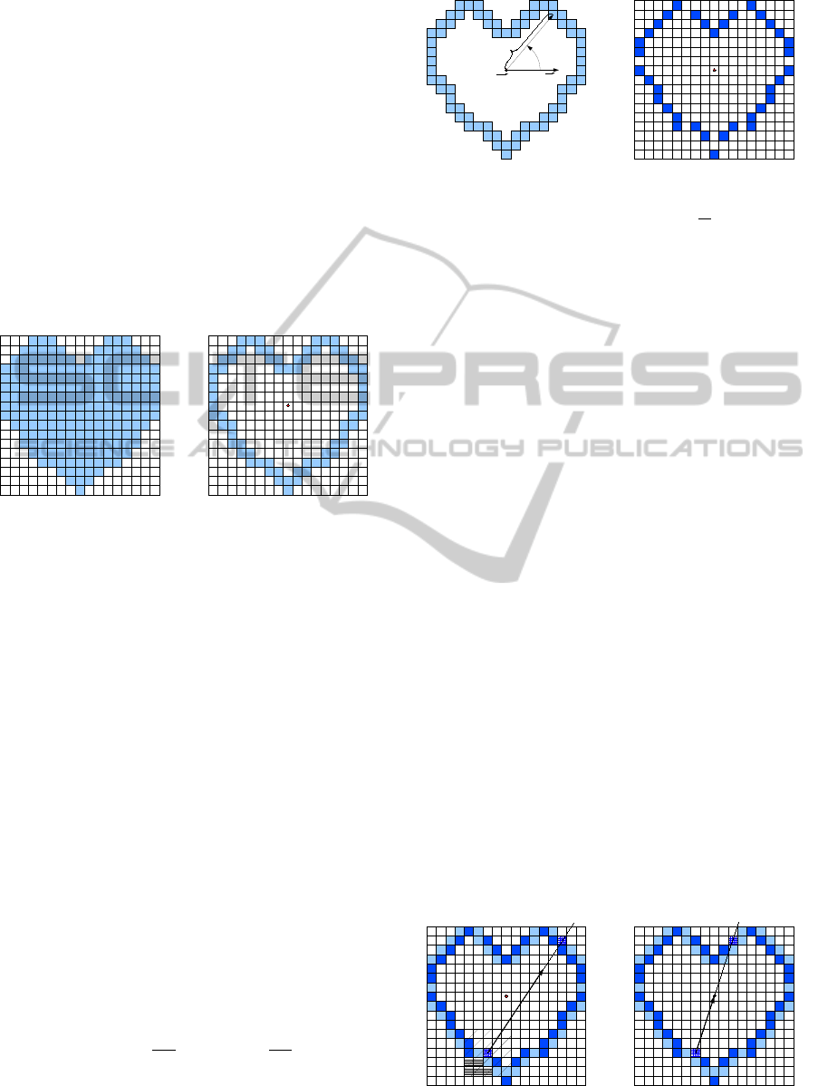
2.1.1 Polar Distance
Fixed angle steps of degree α with 0 < α < 2π, ϕ =
α · n and n = 0, .. . ,d2π/αe − 1 are used to select
individual pixels in A with the maximum distance r to
the centroid s
X
of the segment (see Eq. 3 and Fig. 3).
For non-convex segments, if there is no pixel with the
actual angle ϕ, the pixel with the angle ϕ + π and the
minimum distance to s
X
is chosen. It holds:
s
X
=
x
s
y
s
, x
s
=
1
|X|
|X|
∑
i=1
x
i
, y
s
=
1
|X|
|X|
∑
i=1
y
i
(3)
v
p
= s
X
− p (4)
Φ
r
s
X
ec
.
Figure 3: Polar distance r. Figure 4: Pixel set B se-
lected by the polar dis-
tance, α =
π
18
.
The angle ϕ of a contour point p around s
X
is ∠(v
p
, e)
with the unit vector e = (1 0)
T
, and thus it holds:
v
p
· e = |v
p
| · |e| · cos(ϕ
p
) (5)
All selected pixels are stored in the pixel set B (Fig. 4)
and the distance r of each pixel to the centroid s
X
is stored in the polar distance histogram vector MPD
(maximum polar distance) with a constant number of
elements for each segment.
2.1.2 Contour Signature
In the contour signature histogram vector, MCD
(maximum contour distance), the distance d
N
p
of each
pixel in B to the corresponding opposite pixel in A is
stored. In this case, the straight line between the two
pixels has to have a 90 degree angle to the tangent
through the actual pixel in B.
The direction vector v
CN
to the corresponding op-
posite pixel is approximated by the 24-neighborhood
of the actual pixel p (Fig. 5, Eq. 6, with n = 1 for the
24-neighborhood). This means, we consider a square
of 5× 5 pixels with p as midpoint. The corresponding
opposite pixel a ∈ A is the pixel with biggest distance
to p on v
CN
. MCD has the same cardinality as MPD.
v
CN
=
x
p
+1+n
∑
x
q
=x
p
−1−n
y
p
+1+n
∑
y
q
=y
p
−1−n
p −
x
q
y
q
∀n,q :
q /∈ X ,
n ∈ N (fix)
0
0
otherwise
(6)
Figure 5: Contour signa-
ture.
Figure 6: Ray distance.
SEMANTIC OBJECT RECOGNITION USING CLUSTERING AND DECISION TREES
671
2.1.3 Ray Distance
In the ray distance histogram, the distance d
C
p
of each
Pixel in B to the corresponding pixel in A like in Fig. 6
is stored. Here, the centroid s
X
is on the straight line
between the two pixels and the result is a distance his-
togram vector MCCD (maximum center contour dis-
tance) with the same cardinality as MPD.
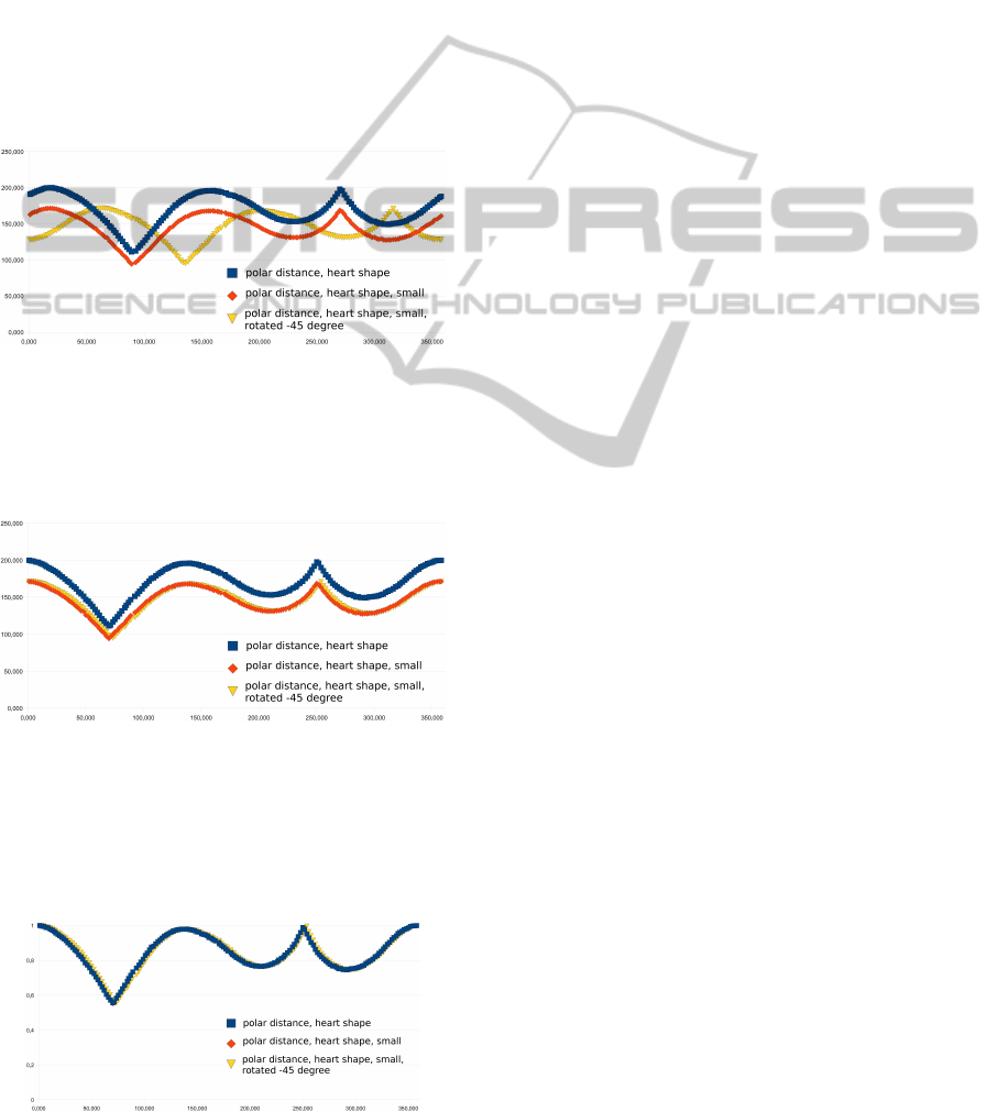
2.1.4 Histogram Normalization
In most cases, the distance histograms have different
values even for the same segment, when this is rotated
or resized (Fig. 7).
Figure 7: Polar distances of three heart shapes.
To get a normalized segment feature vector, each dis-
tance histogram has to be normalized. At first, the ro-
tation is normalized (Fig. 8).
Figure 8: Polar distances with normalized rotation.
In a second step, the values itself are normalized to the
range between 0.0 and 1.0, by dividing the original
distance values by the respective maximum distance
value (Fig. 9).
Figure 9: Polar distances with normalized rotation and size.
After the normalization, all three distance vectors will
joined. Now the feature vector V of the segment is
invariant against translation, rotation and resizing.
2.2 Clustering
In order to reduce the number of feature vectors, a
k-means clustering algorithm is used to build a clus-
ter model (Berry and Linoff, 1997; Han and Kamber,
2006). Each resulting cluster represents a set of simi-
lar feature vectors, and the trained cluster model can
be used to decide the cluster affiliation for a new given
feature vector.
2.3 Decision Trees
For all segments in one image, the clusters for each
segment and its adjacent segments are computed and
stored in a sample vector together with the object cat-
egory of the image. This is done for all downloaded
training images. With this sample vectors a decision
tree model is trained (Berry and Linoff, 1997; Han
and Kamber, 2006). Finally, the trained decision tree
model is used to decide which object is described by
the given sample vector.
3 APPLICATION
3.1 Semantic Robot Vision Challenge
To test the algorithms in a challenging field of ap-
plication, they were implemented for the Semantic
Robot Vision Challenge 2009 (SRVC, 2009).
In this challenge, a robot has 2 hours to find image
examples on the Internet and to learn visual models
for 20 objects, given as a text list. After that, the ob-
jects have to be identified in the environment within
30 minutes without an Internet connection (45 images
were provided in the software league).
3.1.1 Implementation
The presented algorithms were implemented in the
programming language C++ using the OpenCV li-
brary (OpenCV, 2010).
To get the segments of the digital images, an im-
age pyramid segmentation algorithm in OpenCV is
employed (Bradski and Kaehler, 2008). The computa-
tion of the contours and the segment feature vectors is
implemented by the first author. The k-means cluster-
ing of the feature vectors can be done with OpenCV,
but building the cluster model has been implemented
ICAART 2011 - 3rd International Conference on Agents and Artificial Intelligence
672

by the first author, additionally. The OpenCV deci-
sion tree model implementation was used to learn the
object classification with the sample vectors.
3.1.2 Processing the Data and Evaluation
In detail, the concretely implemented procedure
works as follows. Here, all constants are experimen-
tally determined to train the models in less than the
given 120 minutes and to classify the provided images
in less than 30 minutes.
Step 1: Training. Up to 25 images were down-
loaded from the Internet for each object on the list. All
downloaded images were segmented by color and for
each resulting segment, 39083 segments altogether, a
feature vector V with 300 entries was computed (car-
dinality of MPD, MCD and MCCD = 100). After the
association of the feature vectors to 1000 clusters with
k-means clustering, the cluster model is build from the
cluster associations.
Using the cluster model the decision tree model is
trained with a sample vector for each segment struc-
tured as follows: Each sample vector has k + 2 entries
(i.e. chosen cluster count +2). The first k entries con-
tain the number of segments associated to the respec-
tive cluster in the neighborhood of the actual segment
of the image. In this context, neighborhood means that
the bounding boxes of the segments overlap or have
a distance less than 3 pixels. The entry k + 1 contains
the cluster number of the actual segment and the value
of the entry k + 2 is the category identifier of the ac-
tual category of the image.
Step 2: Classification of the Unknown Images.
For each segment in the image the feature vectors V
and the sample vectors are created (without the cate-
gory of the image). The decision tree model predicts
the image category with the sample vectors. Each pre-
dicted category of the image and the number of seg-
ments in the neighborhood of the actual segment is
stored. The category with the most number of seg-
ments in the neighborhood is chosen as the category
of the image.
During the challenge one image was classified
correctly, 14 images were falsely classified and for the
remaining 30 images no category was found (on 9 im-
ages there was not any classifiable object).
4 FUTURE WORK
Our first results are encouraging, but in the future, the
implementation of our approach has to be faster with
an increased object recognition success rate.
For that, the image preprocessing and the segmen-
tation algorithm have to be improved, in order to sup-
port a better classification. Smoothing the distance
histograms to reduce measurement artifacts, using a
clustering algorithm with a variable cluster count to
get a cluster model with less but more precise clusters
and using more spatial relations of the segments for a
more accurate decision tree model is also desirable.
The goal is to implement the approach as a
real-time object recognition system feasible for au-
tonomous multi-copters, i.e. flying robots with several
propellers.
REFERENCES
Alegre, E., Alaiz-Rodrguez, R., Barreiro, J., and Ruiz, J.
(2009). Use of contour signatures and classification
methods to optimize the tool life in metal machining. Es-
tonian Journal of Engineering, 1:3–12.
B
¨
assmann, H. and Kreyss, J. (2004). Bildverarbeitung Ad
Oculos. Springer, Berlin, Heidelberg, New York, 4th edi-
tion.
Berry, M. J. A. and Linoff, G. (1997). Data Mining:
Techniques For Marketing, Sales, and Customer Support.
John Wiley & Sons Inc., New York, Chichester, Wein-
heim, Brisbane, Singapore, Toronto.
Bradski, G. and Kaehler, A. (2008). Learning OpenCV:
Computer Vision with the OpenCV Library. O’Reilly
Media Inc., Beijing, Cambridge, Farnham, K
¨
oln, Se-
bastopol, Taipei, Tokyo.
Han, J. and Kamber, M. (2006). Data Mining: Concepts and
Techniques. Morgan Kaufman Publishers, Amsterdam,
Boston, Heidelberg, London, New York, Oxford, Paris,
San Diego, San Francisco, Singapore, Sydney, Tokyo,
2nd edition.
J
¨
ahne, B. (2005). Digitale Bildverarbeitung. Springer,
Berlin, Heidelberg, New York, 6th edition.
OpenCV (2010). OpenCV (open source computer vision)
library. http://opencv.willowgarage.com/wiki/.
Shuang, F. (2001). Shape representation and retrieval using
distance histograms. Technical report, Dept. of Comput-
ing Science, University of Alberta.
SRVC (2009). Semantic robot vision challenge.
http://www.semantic-robot-vision-challenge.org.
Steinm
¨
uller, J. (2008). Bildanalyse. Von der Bildver-
arbeitung zur r
¨
aumlichen Interpretation von Bildern.
Springer, Berlin, Heidelberg.
SEMANTIC OBJECT RECOGNITION USING CLUSTERING AND DECISION TREES
673
