
Bone Surface Segmentation in Ultrasound Images:
Application in Computer Assisted Intramedullary
Nailing of the Tibia Shaft
Agn`es Masson-Sibut
1,2
, Eric Petit
2
, Franc¸ois Leitner
1
, Julien Normand
3
Amir Nakib
2
and Jean-Baptiste Pinzuti
1
1
Aesculap Research Center, Parc Sud Galaxie, 1 place du Verseau
38432 Echirolles, France
2
LISSI, Universit´e Paris-Est Cr´eteil, 61 Avenue du G´en´eral de Gaulle
94010 Cr´eteil Cedex, France
3
Universit´e de Reims Champagne-Ardenne, 51 rue Cognacq Jay
51095 Reims Cedex, France
Abstract. This paper deals with the use of ultrasound images in order to develop
a Computer Assisted Orthopaedics Surgery system. Ultrasounds are easy to use
in the Operating Room (OR), less expensive than other image modalities, and
faster. We present an automatic method to extract anatomical landmarks from
ultrasound images of femoral anterior condyles. The algorithm is based on an ac-
tive contour model that uses an attraction field derived from an Euclidian-distance
map. This segmentation process is a part of a global procedure that includes an
interactive determination of the best image that could be chosen in order to obtain
robust bone segmentation. This global procedure has been successfully tested on
11 volunteers.
1 Introduction
Ultrasound (US) images are often used in different images analysis procedures in med-
ical field. For example, in cardiology for automatically segmenting and tracking the left
ventricle : using snakes based on a mapping of intensity gradient [11], with a boundary
estimation algorithm using a Bayesian framework [10], using an adaptive version of the
fast marching level set algorithm [15] or developing an artificial neural network (ANN)
method [2]. Or, it can be used in the detection of breast cancer to distinguish benign
masses from malignant cancerous masses, with a threshold based method [6], a Neural
Network (NN) based method [3] or an expectation-maximization method [13].
When it comes to orthopaedic surgery, it is more difficult to use US images due
to several properties of the ultrasounds. Nevertheless, more and more studies had been
conducted to find a robust bone extraction from ultrasound images. It can be used to
register preoperative scans or MRI to the actual human anatomy in the OR [1], to recon-
struct directly the 3D surface of the bone [16], or to test mechanical properties of bones
Masson-Sibut A., Petit E., Leitner F., Normand J., Nakib A. and Pinzuti J..
Bone Surface Segmentation in Ultrasound Images: Application in Computer Assisted Intramedullary Nailing of the Tibia Shaft.
DOI: 10.5220/0003307600340042
In Proceedings of the 2nd International Workshop on Medical Image Analysis and Description for Diagnosis Systems (MIAD-2011), pages 34-42
ISBN: 978-989-8425-38-6
Copyright
c
2011 SCITEPRESS (Science and Technology Publications, Lda.)

non-invasively [9]. In our case, we want to develop a Computer Assisted Orthopaedics
Surgery (CAOS) dedicated to intramedullary nailing for the reconstruction of tibia in
case of shaft fractures. This implies to help the surgeon to detect some anatomical struc-
tures that have been defined in a preceding clinical part of this research project [12].
Few methods have been developed to extract structures in US images. Foroughi et
al. (2007) [4] developed a dynamic programming method using well known features of
the US images to extract the bone interface but it does not lead to very accurate results
because they assume the bone interface as composed of the brightest pixels. This can
cause errors localization of the bone interface up to 4 mm in depth [7].
Hacihaliloglu et al. (2008) [5] developed a method to segment the bone surface and
to detect fractures in 3D US images using 3D local features. The localization accu-
racy and mean errors in estimating fractures displacement are pretty good. Although,
in CAOS systems, the probe usually used is a 2D probe because of the difficulty to
interpret 3D ultrasound images when you are not accustomed to use ultrasounds, and
because of the cost of such a device.
The paper is organized as follow, first we explain how we want to use bone interface
segmentation in the development of a CAOS system. Then, the method of segmentation
using active contours will be developed with some results.
2 Segmentation of the Bone Interface
Our final goal is to develop a CAOS system to help orthopaedic surgeon to perform
intramedullary nailing in case of treatment of tibia shaft fractures. In case of tibia shaft
fractures, orthopaedic surgeons can use plates, intramedullary nail, or extern fixation
as treatment. When intramedullary nailing is chosen, the surgeon determines the length
and orientation of the leg, only basing himself on its own expertise. Such a decision is
critical.
Once the nail is in place, the assistance system we developed will help the surgeon
to respect the most the anatomy of the patient. To do so, long bones are considered
symmetrically similar [12]. Two 3D models (one for the healthy member and one for
the injured one) are built using some anatomical landmarks located whether by man-
ual pointer or US probe. These landmarks are the two malleolus and the distal site of
fracture for the distal part of models, and the middle of the trochlea, the condylar line
and the proximal site of fracture for the proximal part of models. These one are located
with the leg in full extension. Thus, the tibia is locked regarding to the femur, and we
can use the femoral frame of reference to orientate the tibia. Then, the system guides
the surgeon to fix the fracture such as finally, the two models fit.
Some of anatomical points are located using a manual pointer because they are near
the skin. It is not the case for the middle of the trochlea, and the condylar line. We use
ultrasound images and we extract these features automatically.
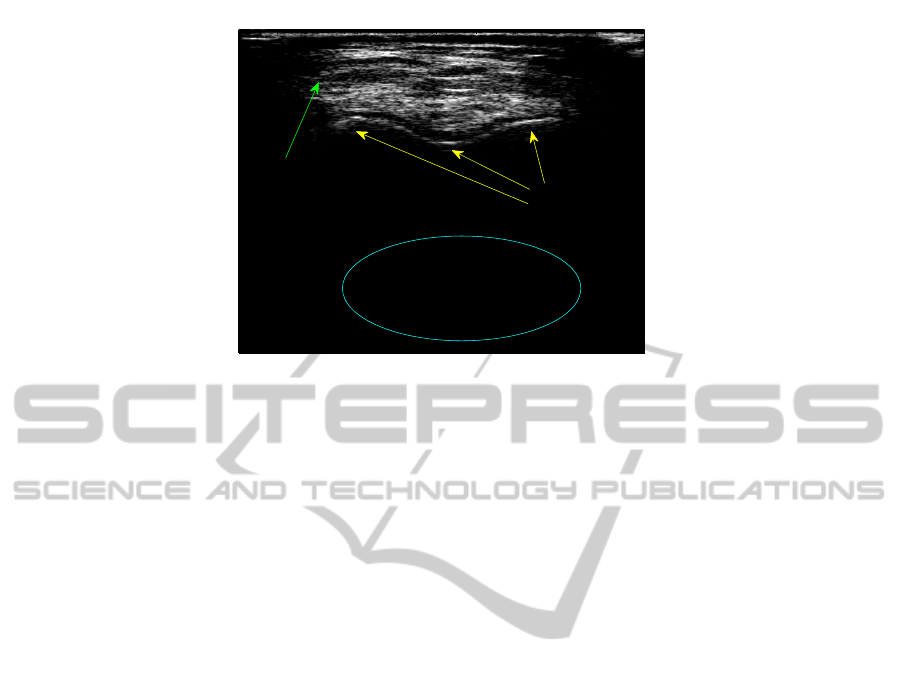
Figure 1 shows an US image of the femoral condyles (the interface between bone
and tissue is highlighted).
The bone interface in the image represents the interface between soft tissue and
femoral anterior condyles, and the shadow is the non-echo zone under the bone inter-
face . Due to the frequency of US in orthopaedics, waves cannot penetrate the bone
35
50 100 150 200 250 300 350 400 450 500
50
100
150
200
250
300
350
400
450
500
Shadow
Bone surface
Soft tissue
Fig.1. An ultrasound image of the femoral condyles. We can easily distinguish the bone interface
and the shadow that represents the non-echo zone under the bone.
surface. This shadow feature is very important because it is a constant in US images of
bone. In our method, it is used to initialize automatically the contour. Anothercharacter-
istic about US imaging of the bone is that the bone interface is very bright in the image.
But, because the US waves and echoes propagate like spherical waves, the resolution is
not very good and the interface thickness can reach over than 4mm [7]. According to
Jain and Taylor, it is more likely that the bone interface lies on the top of the fiducial
surface. We take that into account when we calculate the distance map.
To be able to compare 3D models of the injured and the healthy tibia, we have to
define a precise protocol of acquisition for the US images. In our case, the surgeon put
the probe just under the patella with a full extension leg. Thus, the US probe is locked
by the patella. Then, the surgeon has to scan the anterior condylar profile and the CAOS
system finds the image perpendicular to the bone surface and extract the landmarks we
want from it.
2.1 Proposed Method
US images have a high level of speckle and intensity dropouts. Thus, to avoid segmen-
tation troubles and to have a continuous contour, we proposed to use an active contour
model. This class of methods was introduced by Kass et al. [8], forces are applied to an
initial curve causing its deformation and displacement until it reaches an equilibrium
state.
The evolution of the snake is based on a minimization of the energy along the curve.
Then, we define the total energy E
snake
as:
E
snake
=
n
X
1
E
int
(i) + E
ext
(i) (1)
The internal energy (E
int
) is derived from the properties of the curve and is defined by
36
50 100 150 200 250 300 350 400 450 500
50
100
150
200
250
300
350
400
450
500
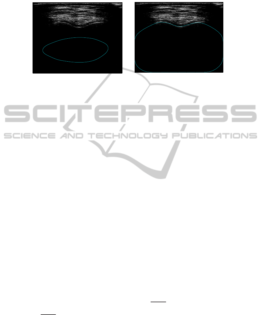
(a)
50 100 150 200 250 300 350 400 450 500
50
100
150
200
250
300
350
400
450
500
(b)
Fig.2. Movement of the snake. (a) Initial contour (b) Stabilized snake.
E
int
= α(s)kν
s
(s)k
2
+ β(s)kν
ss
(s)k
2
(2)
where α(s) controls the tension of the curve (the curve acts like a membrane), β(s)
controls the rigidity, and ν(s) = (x(s), y(s)) with s the curvilinear abscissa. In this
paper, we propose a new expression of the external energy that is more adapted to our
application. This energy is based on constrained euclidian map transform.
Firstly, we propose to apply a Derivative of Gaussian (DoG) filter to the original
image
I
grad
= ∆(G
σ
∗ I) (3)
Then, we threshold the cumulative histogram of the intensities ( I
grad
), and keep only
the 3% highest values.
I
BW
= H
cumul
3%
(I
grad
) (4)
At this step, we have a binary image. The following step consists to use a com-
bination of morphological operations to close the area where there are some gradient
points. Morphological filters are whether erosion (ǫ
E
) or dilatation (δ
E
) with a struc-
turing element E which is a binary mask. These filters can be combined to give closure
(I •E = ǫ
E
δ
E
(I)) or opening (I ◦E = δ
E
ǫ
E
(I)). In our case, we perform two closures
with oblique lines to close the two condylar slopes, and to close the logical sum with a
disk element.
I
Mask
= ((I
BW
• E
(line,85,155)
) ∨ (I
BW
• E
(line,85,25)
)) • E
(disk,15)
(5)
Thus, for line elements, the second argument is the length, and the third is the orienta-
tion. For the disk element, the second argument is the radius. The result image I
Mask
is a binary mask. Afterwards, we use this mask to calculate the Euclidian distance map
that attracts the active contour curve on condylar contours.
E
ext
= dist(I
Mask
) + dist(I
Mask
) (6)
where I
Mask
is the negation of I
Mask
.
37

In the next section, we present the 3 step procedure that we use. The first step is
the initialization of the contour on the image chosen by the user. The second step is the
tracking of the bone interface in a serie of US images, and the automatic choice of the
particular image. Finally, the system extracts the landmarks from this image.
2.2 Snake Initialization
The initialization of the snake is performed on an image chosen by the user, where a
visible interface between soft tissue and bone appears. It is known that there is a black
shadow under the bone surface, we initialize the active segmentation process by placing
a closed curve in this part of the image. Then, we determine the forces to be applied
to the curve so it can move to fit the bone interface. The internal force (E
int
) controls
stiffness and elasticity of the curve. We choose parameters that allows the curve to
move without depending on intensity dropouts (high stiffness) and the evolution is fast
enough (high elasticity).
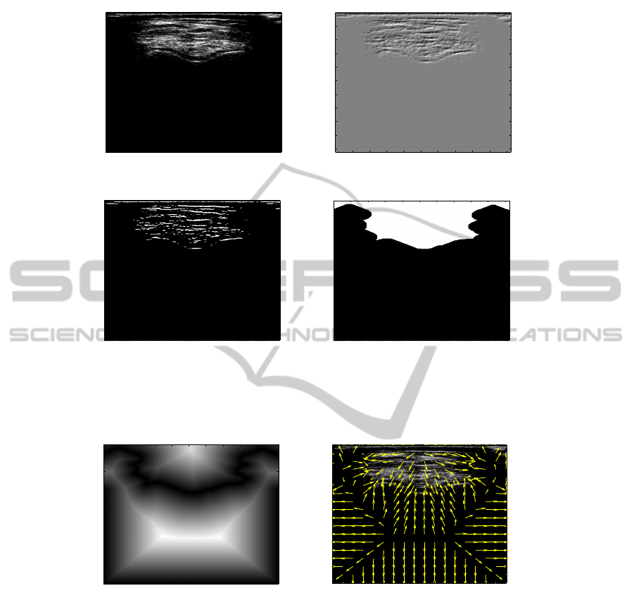
In order to define the external force, we calculate a constrained Euclidian distance
map on a binary mask. For that, we perform a rough regional segmentation of the
light part of the image that corresponds to soft tissues. As we explained in previous
part, a smoothed gradient is applied by using a Derivative of Gaussian (DoG) opera-
tor (Fig. 3.b). The resulting image is then thresholded to keep only significant contour
points (Fig. 3.c). Finally the rough regional segmentation is obtained by a morphologi-
cal closing of the gradient binary image (Fig. 3.d).
Thus we obtain the E
ext
image calculating the Euclidian distance transform (Fig-
ure 4.a). Figure 4.b shows the corresponding field of attraction of the active model
contour that leads to the final result (Fig. 2.d). This final contour will serve to track the
bone surface in a serie of images.
2.3 Tracking of the Bone Surface
After the initial detection of the bone interface , the surgeon scans the region of anterior
condyles in order to find an optimal cross-section to the bone surface.
In this procedure, for each new image, the contour detection process is the same than
for the initial detection described in the preceding section, except that the initialization
of the active curve is realized using the last detected bone surface. Then, to assist the
surgeon in this localization, we sum the intensities along the newly detected contour for
each new acquired image ; the maximum value is obtained for the optimal cross-section
(Fig. 5).
Then, we extract landmarks we are interested in from the result image.
2.4 Finding Particular Landmarks
The landmarks the system has to extract are the middle of the trochlea, and top of both
anterior condyles to define the condylar line. This line allows us to orientate the 3D
model of the tibia.
Due to parameters we used for our snake, we can find our landmarks on local maxi-
mum for both top of condyles,and local minimum for the middle of the trochlea (Fig. 6).
38
50 100 150 200 250 300 350 400 450 500
50
100
150
200
250
300
350
400
450
500
(a)
50 100 150 200 250 300 350 400 450 500
50
100
150
200
250
300
350
400
450
500
(b)
50 100 150 200 250 300 350 400 450 500
50
100
150
200
250
300
350
400
450
500
(c)
50 100 150 200 250 300 350 400 450 500
50
100
150
200
250
300
350
400
450
500
(d)
Fig.3. Determination of a mask image (a) initial image, (b) filtered image by a Derivative of the
Gaussian, (c) thresholded and filtered image (d) mask image resulting from a closing operation
applied on the binary image.
50 100 150 200 250 300 350 400 450 500
50
100
150
200
250
300
350
400
450
500
(a)
50 100 150 200 250 300 350 400 450 500
50
100
150
200
250
300
350
400
450
500
(b)
Fig.4. Field of attraction using to calculate external energy (a) Euclidian distance map used to
calculate the field of attraction for the snake (b) Initial image with the field of attraction/repulsion
superimposed.
3 Results
The algorithm has been tested on 36 series of images for 11 healthy femurs. First results
demonstrate the validity of the global procedure. The populatio used to test the algo-
rithm is constituted of men and women, from 24 to 40 year-old, and both right and left
knees. Our validation is only qualitative, but 26 series gave a good result. So, 10 series
39
50 100 150 200 250 300 350 400 450 500
50
100
150
200
250
300
350
400
450
500
Fig.5. Result of snake evolution.
50 100 150 200 250 300 350 400 450 500
50
100
150
200
250
300
350
400
450
500
Fig.6. Extraction of Points of Interest from the chosen image.
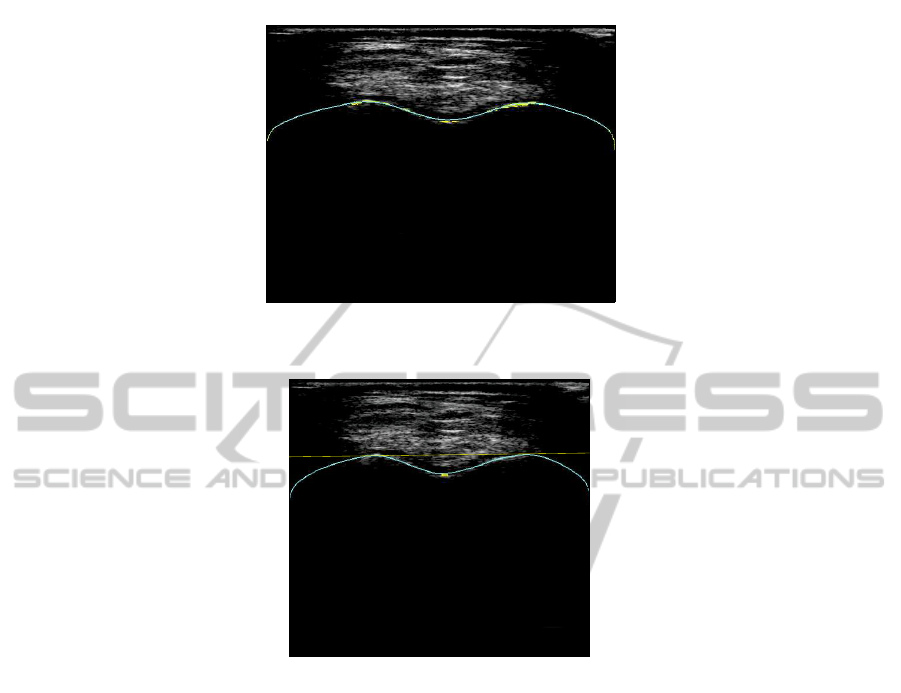
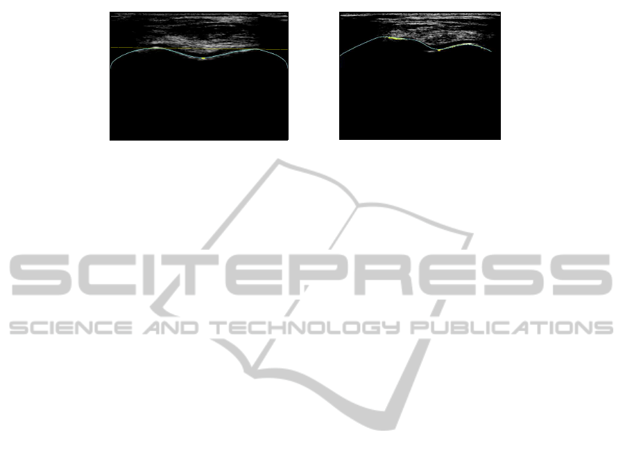
provide bad results because the acquisition did not follow strictly the protocol. Some
cases, like the image 7.b gives bad result due to the US profile shape. On the contrary,
image 7.a shows a good result.
The execution time is approximately 0.5 second per image. The algorithm has been
implemented on Matlab
R
, and tested on a computer with a Dual-Core Intel
R
CPU
(E5200 at 2.50GHz) and 1Go RAM, and the XP SP3 version of Windows
R
.
4 Conclusions and Perspectives
We proposed a method to extract the bone surface from US images of the femoral
condyles, and we applied this method in a CAOS system assisting the surgeon per-
forming intramedullary nailing as treatment of tibia shaft fractures. This method can be
used to segment bone surface in other types of images such as for iliac crest, and it can
also be used in some other kind of surgery, like computer assisted osteotomy. In work
under progress is a demonstrator of our CAOS system in the context of an Operating
40
50 100 150 200 250 300 350 400 450 500
50
100
150
200
250
300
350
400
450
500
(a)
50 100 150 200 250 300 350 400 450 500
50
100
150
200
250
300
350
400
450
500
(b)
Fig.7.Some results of landmarks extraction. (a) Good detection of landmarks. (b) False detection.
Room. A use of General-purpose Processing on Graphics Processing Units (GPGPU)
to accelerate calculus is also under progress to be able to run our method on real time.
We also want to extend this work to assist the surgeon on other kind of orthopaedic
surgery (concerning iliac crest for instance).
References
1. D. Amin, T. Kanade, A. M. D. Gioia, and B. Jaramaz. Ultrasound Registration of the Bone
Surface for Surgical Navigation. Computer Aided Surgery, (1):1–16, 2003.
2. T. Binder, M. S¨ussner, D. Moertl, T. Strohmer, H. Baumgartner, G. Maurer, and G. Porenta.
Artificial neural networks and spatial temporal contour linking for automated endocardial
contour detection on echocardiograms: a novel approach to determine left ventricular con-
tractile function. Ultrasound in medicine & biology, 25(7):1069–76, Sept. 1999.
3. D.-R. Chen, R.-F. Chang, W. Kuo, M. Chen, and Y. Huang. Diagnosis of breast tumors
with sonographic texture analysis using wavelet transform and neural networks. Ultrasound
Medical Biology, 30(5):1301–1310, Apr. 2002.
4. P. Foroughi, E. Boctor, M. J. Swartz, R. H. Taylor, and G. Fichtinger. Ultrasound Bone Seg-
mentation Using Dynamic Programming. 2007 IEEE Ultrasonics Symposium Proceedings,
pages 2523–2526, Oct. 2007.
5. I. Hacihaliloglu, R. Abugharbieh, A. Hodgson, and R. Rohling. Bone segmentation and
fractire detection in ultrasound using 3D local phase features. MICCAI 2008, pages 287–
295, 2008.
6. K. Horsch, M. L. Giger, L. A. Venta, and C. J. Vyborny. Automatic segmentation of breast
lesions on ultrasound. Medical physics, 28(8):1652–9, Aug. 2001.
7. A. K. Jain. Understanding bone responses in B-mode ultrasound images and automatic
bone surface extraction using a Bayesian probabilistic framework. Proceedings of SPIE,
5373:131–142, 2004.
8. M. Kass, A. Witkin, and D. Terzopoulos. Snakes: Active contour models. International
Journal of Computer Vision, 1(4):321–331, Jan. 1988.
9. P. Laugier, F. Padilla, F. Peyrin, K. Raum, A. Saied, M. Talmant, and L. Vico. Current trends
in ultrasonic investigation of bone. ITBM-RBM, 26:299–311, 2005.
10. M. Mignotte, J. Meunier, and J.-C. Tardif. Endocardial Boundary Estimation and Tracking in
Echocardiographic Images using Deformable Template and Markov Random Fields. Pattern
Analysis & Applications, 4(4):256–271, Nov. 2001.
11. A. Mishra. A GA based approach for boundary detection of left ventricle with echocardio-
graphic image sequences. Image and Vision Computing, 21(11):967–976, Oct. 2003.
41

12. J. Normand. Approche exp´erimentale de la navigation dans les fractures de la jambe. PhD
thesis, Facult´e de M´edecine, Universit´e de Reims, FRANCE, 2009.
13. G. Xiao, M. Brady, J. A. Noble, and Y. Zhang. Segmentation of ultrasound B-mode images
with intensity inhomogeneity correction. IEEE transactions on medical imaging, 21(1):48–
57, Jan. 2002.
14. C. Xu and J. L. Prince. Gradiant Vector Flow : A new external force for snakes. IEEE
Proceedings Conference on Computer Vision Pattern Recognition, pages 66–71, 1997.
15. J. Yan and T. Zhuang. Applying improved fast marching method to endocardial boundary
detection in echocardiographic images. Pattern Recognition Letters, 24(15):2777, 2003.
16. Y. Zhang, R. Rohling, and D. Pai. Direct surface extraction from 3D freehand ultrasound
images. In Proceedings of the conference on Visualization’02, page 52. IEEE Computer
Society, 2002.
42
