UNSUPERVISED LEARNING FOR TEMPORAL SEARCH SPACE
REDUCTION IN THREE-DIMENSIONAL SCENE RECOVERY
Tom Warsop and Sameer Singh
Research School of Informatics, Holywell Park, Loughborough University, Leicestershire, LE11 3TU, U.K.
Keywords:
Three-dimensional scene recovery, Search space reduction, Unsupervised learning.
Abstract:
Methods for three-dimensional scene recovery traverse scene spaces (typically along epipolar lines) to com-
pute two-dimensional image feature correspondences. These methods ignore potentially useful temporal in-
formation presented by previously processed frames, which can be used to decrease search space traversal.
In this work, we present a general framework which models relationships between image information and
recovered scene information specifically for the purpose of improving efficiency of three-dimensional scene
recovery. We further present three different methods implementing this framework using either a naive Near-
est Neighbour approach or a more sophisticated collection of associated Gaussians. Whilst all three methods
provide a decrease in search space traversal, it is the Gaussian-based method which performs best, as the other
methods are subject to the (demonstrated) unwanted behaviours of convergence and oscillation.
1 INTRODUCTION
Recovering three-dimensional (3D) scene informa-
tion from two-dimensional (2D) image information
can be very useful. The work presented in this paper
is part of a larger project concerned with recovering
3D scene information from a train mounted, forward-
facing camera.
Many methods have previously been applied to
3D scene recovery. As highlighted by (Favaro et al.,
2003), a large proportion of these methods follow a
similar pattern of execution. First point-to-point cor-
respondences among different images are established.
These image correspondences are then used to in-
fer three-dimensional geometry. These feature cor-
respondences can be computed in one of two ways,
either by seaching the 2D image plane or by incorpo-
rating epipolar geometry.
The first set of methods do not take the 3D na-
ture of the problem into account. These methods typ-
ically operate in two steps. First, image features are
detected. Methods presented in literature use Har-
ris corners ((Li et al., 2006)), SIFT features ((Zhang
et al., 2010)) and SURF features ((Bay et al., 2008)).
More recently, to compensate for viewpoint changes
in captured image information (Chekhlov and Mayol-
Cuevas, 2008) artifically enhanced the feature set for a
single image point considered, computing spatial gra-
dient descriptors for multiple affine transformed ver-
sions of the image area surrounding a feature point.
Feature correspondences are then computed by fea-
ture matching in subsequent frames.
It is, however, possible to incorporate 3D informa-
tion into these feature correspondence computations.
One of the most straightforward ways of integrating
3D information uses stereo cameras. Under schemes
such as these, as can be seen in the work of (Zhang
et al., 2009; Fabbri and Kimia, 2010; Li et al., 2010)
and (Grinberg et al., 2010) (to name a few) epipo-
lar scanlines across left and right-hand images are
searched for matching feature correspondence. It is
possible to integrate these concepts into monocular
camera configurations such as in the method intro-
duced by (Klein and Murray, 2007) known as Paral-
lel Tracking and Mapping (PTAM). In which features
are initialised with their 3D positions by searching
along epipolar lines, defined by depth between key
frames of the image sequence. (Davison, 2003; Davi-
son et al., 2007) presented a similar idea of feature
initialisation in monoSLAM.
When recovering 3D information from image se-
quences, if they are processed in reverse chronologi-
cal order new scene elements to process appear at im-
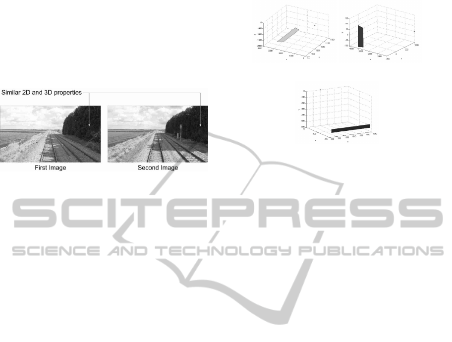
age edges. This provides an interesting property - im-
age areas recovered in subsequent image frames ex-
hibit similar properties to those processed previously,
highlighted in Figure 1. It may therefore be possi-
ble to exploit this information, using relationships be-
549
Warsop T. and Singh S..
UNSUPERVISED LEARNING FOR TEMPORAL SEARCH SPACE REDUCTION IN THREE-DIMENSIONAL SCENE RECOVERY.
DOI: 10.5220/0003308405490554
In Proceedings of the International Conference on Computer Vision Theory and Applications (VISAPP-2011), pages 549-554
ISBN: 978-989-8425-47-8
Copyright
c
 2011 SCITEPRESS (Science and Technology Publications, Lda.)

tween 2D image features and recovered 3D scenes to
reduce the size of the search spaces traversed (for ex-
ample, along epipolar lines) when computing feature
correspondences. Such a concept has not been pro-
posed by previous methods and forms the basis of
the method presented in this work (named Temporal
Search space Reduction, or TSR).
Figure 1: When processing image sequences in reverse or-
der, new scene elements entering at image edges exhibit
similar 2D image and 3D scene properties.
The structure of the remainder of this paper is as
follows. Section 2 presents a brief overview of the 3D
scene recovery method used as a platform for exper-
imental comparison of the TSR extension. The TSR
concept and three implementations are discussed in
section 3. Experimental results regarding real data are
provided in section 4, as is the discussion of problems
faced by methods implementing the TSR concept. Fi-
nally, section 5 concludes the work in this paper.
2 THREE-DIMENSIONAL
SEQUENCE RECOVERY
To demonstrate the TSR concept, the 3D scene recov-
ery method described by (Warsop and Singh, 2010) is
used. This method has been chosen because it can be
simply adapted to recover dense 3D scene informa-
tion in the form of planes, in which correspondences
are searched for along categorized epipolar lines. This
method recovers the 3D corner points of a plane re-
lated to image quadrilaterals by searching for the 3D
corner values which provide the lowest reprojection
error in a subsequent frame. Summarized as:
P
3D
= min
Q
3D
{SAD(S
1
, SQR(R(Q
3D
, I
2
), I
2
))} (1)
where, SAD(x, y) computes the sum-of-absolute dif-
ferences in the RGB channels of images x and y,
R(Q, I) reprojects the 3D coordinates of Q into subse-
quent image I, SQR(q, I) converts a quadrilteral im-
age area q into a square area using image data I,
S
1
= SQR(Q
1
, I
1
) where Q
1
and I
1
are the original
quadrilateral and image under consideration (respec-
tively) and Q
3D
are the 3D coordinates of the quadri-
lateral corner points searched through. The adaptation
(a) Flat. (b) Side.
(c) Vertical.
Figure 2: The three base types of plane used for searching
in the 3D scene recovery method.
made to this method takes the form of only using three
types of planes (shown in Figure 2) when searching
for the best matching plane - defined by height, width
and depth respectively.
3 UNSUPERVISED LEARNING
FOR TEMPORAL SEARCH
SPACE REDUCTION
Figure 3 demonstrates how the concept proposed by
TSR (shaded boxes) integrates with a typical 3D
scene recovery method (unshaded boxes). The fol-
lowing describes each shaded box:
1. Compute 2D Image Features - since the image
area surrounding a feature is to be used to indi-
cate the 3D search space to traverse, these features
must be computed.
2. (2D,3D) Relationship Model - storing the rela-
tionship between 2D image features and corre-
sponding recovered 3D information.
3. Compute 3D Search Space - for any new feature
considered for recovery, the range of 3D values
to consider should be selected based upon the
computed 2D values. If similar features have
been processed before, narrow ranges around ex-
pected values should be searched. Otherwise,
large ranges should be selected. These search
ranges are defined by a category type (flat, ver-
tical or side) and value (height, depth or width).
4. Update the Model - once a new feaure has been
recovered, the model storing the 2D and 3D re-
lationships must be updated to include this new
information.
VISAPP 2011 - International Conference on Computer Vision Theory and Applications
550

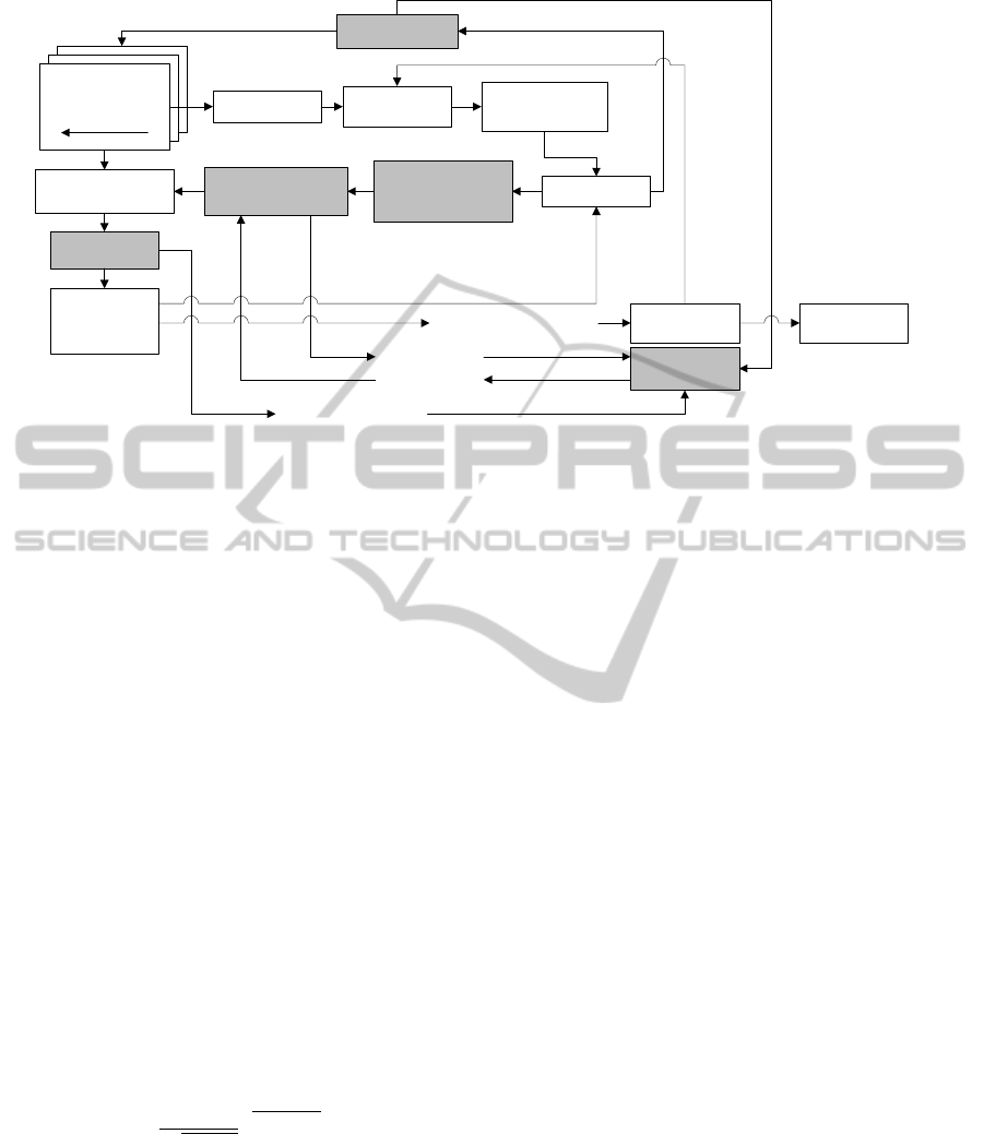
Image sequence Next Image
Recovered 3D
scene
Project current 3D
scene into image
Detect features in
new, unprocessed
image areas
For each feature
(1) Compute 2D image
features from image
area surrounding
feature
(3) Compute 3D search
space range(s) to
traverse
Recover 3D information
related to feature
(4) Update model
Add recovered
feature information
to 3D scene
(2) (2D,3D)
relationship model
2D image features
3D range(s)
2D image features and
recovered 3D information
Recovered 3D information
(5) Degrade model
Output: recovered
3D scene
Figure 3: 3D sequence recovery method (unshaded box) enhancement, incorporating temporal information stored as a rela-
tionship between 2D image information of the area surrounding a feature and corresponding recovered 3D information. The
grey shaded boxes represent the additions proposed by TSR.
5. Model Degradation - it is necessary to degrade
the model on each iteration, preventing it from
consuming too much memory.
The following subsections discuss three different
methods for implementing these proposed TSR exten-
sions. Each method uses the same image features - for
each image quadrilateral area considered separate red,
green and blue histograms are computed. From which
each of the mean, standard deviation, skewness, kur-
tosis and energy are computed, resulting in 15 fea-
tures.
3.1 Nearest Neighbour (NN)
The first implementation stores the (2D,3D) rela-
tionship as a list of tuples (M) of the form: <
2D image features, category, value >. For any newly
processed quadrilateral, the categories to process are
determined by computing the following value for each
category, c ∈ flat, side, vertical:
p
c
=
1
q
2πσ
2
Nc
e
−( f −µ
Nc
)
2
2σ
2
Nc
(2)
where, f are the 2D image features of the currently
considered quadrilateral, Nc represents the K Eu-
clidean nearest neighbours to f in M of category c,
µ
Nc
and σ
Nc
are the mean and standard deviation of
Nc respectively. The resultant set of probabilities are
normalized and any above a threshold indicate the
corresponding categories should be processed. The
range of values to process for any chosen category are
defined by a minimum and maximum value computed
using:
min
c
= µ
v
− (Dσ
v
× (1 − p
c
)) (3)
max
c
= µ
v
+ (Dσ
v
× (1 − p
c
)) (4)
where, µ
v
and σ
v
are the mean and standard deviation
of the 3D values associated with Nc and D is a scalar
value. Scene recovery results are used to create new
tuples to update M with. To implement model degra-
dation, an extra distance field is used in the tuples of
M. When a tuple is added to M, this field is initialised
to zero and accumulates the distance travelled by the
camera since initialisation. A threshold of this dis-
tance field can then be used to remove old tuples.
3.2 Nearest Neighbour with Error
Correction (NNEC)
The second implementation proceeds as the previous
NN method. But with the addition that after recovery
has been performed the SAD value associated with
the best set of quadrilateral corners (BQ
3D
) is com-
puted:
min
SAD
= SAD(S
1
, SQR(R(BQ
3D
, I
2
), I
2
)) (5)
where everything has the same meaning as in Equa-
tion 1. If min
SAD
is greater than a pre-determined
threshold, the value ranges selected for processing by
the nearest neighbour metric are deemed to of been
inappropriate and recovery is performed again, using
all value ranges. The subsequent result is added to the
tuple list as before.
UNSUPERVISED LEARNING FOR TEMPORAL SEARCH SPACE REDUCTION IN THREE-DIMENSIONAL SCENE
RECOVERY
551

3.3 Feature and Value Gaussians (FVG)
The relationship model of this implementation builds
a set of Gaussian distributions for the 2D image fea-
tures encountered. Similar 2D image features are rep-
resented by a single multi-dimensional Gaussian dis-
tribution. Each of these feature distributions is asso-
ciated with value range distributions, each represent-
ing similar 3D values that have been recovered for the
corresponding 2D image features. Each value distri-
bution also has an associated category.
For any new feaure recovered, the probability the
corresponding image features ( f ) belong to any of the
feature distributions are computed:
p
FD
=
1
q
2πσ
2
FD
e
−( f −µ
FD
)
2
2σ
2
FD
(6)
where, p
FD
is computed for each of the feature dis-
tributions, FD is the current feature distribution un-
der consideration and µ
FD
ad σ
FD
are the mean and
standard deviation of FD respectively. For each p
FD
greater than a pre-determined threshold, the associ-
ated value distributions are each considered in turn
and used to determine a value range to process, us-
ing the minimum and maximum computed in a sim-
ilar manner to Equations 3 and 4. If V R represents
the set of all values to process of a new feature, the
best fitting plane for the considered 3D scene recov-
ery method is computed using:
P
3D
= min
Q
3D
∈V R
{SAD(S
1
, SQR(R(Q
3D
, I
2
), I
2
))}
(7)
If the SAD value associated with P
3D
is greater
than a threshold, reprocessing proceeds as for the
NNEC method. Under this scheme, there are three
possible ways in which the model can be updated.
These are demonstrated in Figure 4, where green rep-
resents update and red means a new distribution is
added. Model degradation is performed by storing
a distance since last update with each distribution,
where distance is in terms of camera movement. If
this distance exceeds a threshold the corresponding
Gaussian is removed.
4 EXPERIMENTAL RESULTS
The data used for experimentation consists of high-
definition (i.e. 1920 × 1080 pixels) image frames,
captured from a front-forward facing camera mounted
on a train. In total, 5 sequences totalling 520 im-
age frames were used. Each image frame was ground
truthed by hand - matching approximately 850 fea-
tures between image pairs.
(a) No feature matching.
(b) Feature matching but value reprocessing.
(c) Feature matching and no value reprocessing.
Figure 4: Graphical repesentation of the three different
types of update in FVG.
With regards to TSR methods presented in section
3, Figure 5(a) presents the average number of com-
binations checked per quadrilateral recovered in each
frame and Figure 5(b) the accuracy of each method,
where Exhaustive refers to the unaltered method de-
scribed in section 2. The results show that each of the
methods implementing the TSR extensions provides a
decrease in the number of combinations checked per
recovered quadrilateral whilst maintaining similar ac-
curacy. However, this reduction sometimes comes at
a cost. For example, the NN method produces less
accurate scene recovery results. This is because the
NN relationship model can converge. Consider a syn-
thetic image sequence comprising of only a textured
wall and floor plane such as in Figure 6. The sequence
was created such that in the first 10 images, the wall is
of a fixed x-coordinate of 400. Then in the 19th image
the wall was created with an x-coordinate of 0.
In the first 18 images of the sequence, the whole
image was processed and used to update the NN
model. In the 19th image only a square of the wall
VISAPP 2011 - International Conference on Computer Vision Theory and Applications
552

(a) Average number of quadrilterals checked
per sequence frame.
(b) Average difference between recovered sequence frames and ground
truth.
Figure 5: Comparison of the number of checks made and difference with ground truthed scene per method, averaged over all
5 sequences.
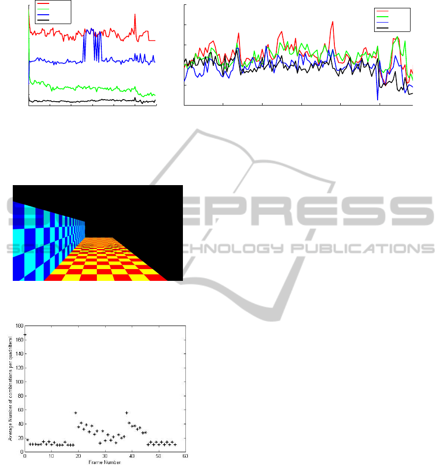
Figure 6: Synthetic image sequence example comprising of
a floor and wall plane.
Figure 7: Number of combinaions procesed by the NNEC
method for the oscillating wall sequence.
plane was recovered. As expected, the side plane cat-
egory was chosen. However, because all previous side
planes processed are of width 400, the value range
chosen to process is 390.50 to 421.04. Clearly this is
incorrect. The error occurs because for a large part of
the sequence one set of 2D image features maps to one
specific 3D value. Hence, the model converges for
these 2D image features. When the 3D value changes
for this specific set of features the model cannot rep-
resent this, resulting in possible error.
NNEC resolves this convergence issue. However
because of the nearest neighbour selection scheme,
this method can produce oscillatory behaviour. For
example, consider a similar synthetic image se-
quence, except in this one the x-coordinate for the
wall is 400 pixels for 20 frames, then 0 for 20 frames
and 400 pixels for a further 20 frames. When the wall
plane value changes for the first time, error correc-
tion is invoked and slowly more correct members are
added to the pool of nearest neighbours, but when the
wall plane value reverts back to the original value the
same process repeats - highlighted in Figure 7.
The FVG method avoids these problems because
the multiple associated value distributions can repre-
sent different values the features have been mapped to
in the sequence so far.
5 CONCLUSIONS
We have presented a general update to 3D scene re-
covery methods which takes advantage of temporal
information to increase efficiency. As such, 3 differ-
ent implementations were provided and applied to an
existing 3D scene recovery method. Of which, the
simple nearest neighbour methods are affected by the
problems of convergence and oscillatory behaviour.
The Gaussian model presented copes well with both
of these problems, reducing the search space traversal
by an order of magnitude and maintaining accuracy
of recovered scenes. Now that we have demonstrated
the advantages and pitfalls of these methods, we wish
to further investigate the benefits of the TSR concept,
integrating it with other methods and applying it to
more challenging data.
UNSUPERVISED LEARNING FOR TEMPORAL SEARCH SPACE REDUCTION IN THREE-DIMENSIONAL SCENE
RECOVERY
553

REFERENCES
Bay, H., Ess, A., Tuytelaars, T., and Gool, L. V. (2008).
Surf: Speeded up robust features. Computer Vision
and Image Understanding (CVIU), 110(3):346–359.
Chekhlov, D. and Mayol-Cuevas, W. (2008). Appearance
based indexing for relocalisation in real-time visual
slam. In 19th British Machine Vision Conference,
pages 363–372.
Davison, A. J. (2003). Real-time simulataneous localization
and mapping with a single camera. In Proc. Interna-
tional Conference on Computer Vision, pages 1403–
1411.
Davison, A. J., Reid, I. D., Molton, N. D., and Stasse, O.
(2007). Monoslam: Real-time single camera slam. In
IEEE Transactions on Pattern Analysis and Machine
Intelligence, volume 29, pages 1–15.
Fabbri, R. and Kimia, B. (2010). 3d curve sketch: Flexible
curve-based stereo reconstruction ad calibration. In
2010 IEEE Conference on Computer Vision and Pat-
tern Recognition, pages 1538–1545.
Favaro, P., Jin, H., and Soatto, S. (2003). A semi-direct ap-
proach to structure from motion. In The Visual Com-
puter, volume 19, pages 377–384.
Grinberg, M., Ohr, F., and ad J. Beyerer, D. W. (2010).
Feature-based probabilistic data association and track-
ing. In The 7th International Workshop on Intelligent
Transportation (WIT2010), pages 29–34.
Klein, G. and Murray, D. (2007). Parallel tracking and map-
ping for small ar workspaces. In Proceedings and
the Sixth IEEE and ACM International Symposium on
Mixed and Augmented Reailty (ISMAR07).
Li, J., Li, ., Chen, Y., Xu, L., and Zhang, Y. (2010). Bun-
dled depth-map merging for multi-view stereo. In
2010 IEEE Conference on Computer Vision and Pat-
tern Recognition, pages 2769–2776.
Li, P., Farin, D., Gunnewiek, R. K., and de With, P. H. N.
(2006). On creating depth maps from monoscopic
video using structure frm motion. In 27th Symposium
on Information Theory, pages 508–515.
Warsop, T. E. and Singh, S. (2010). Robust three-
dimensional scene recovery from monocular image
pairs. In 9th IEEE International Conference on Cy-
bernetic Intelligent Systems 2010 (CIS 2010), pages
112–117.
Zhang, G., Dong, Z., Jia, J., Wong, T.-T., and Bao, H.
(2010). Efficient non-consecutive feature tracking for
structure-from-motion. In ECCV 2010, pages 422–
435.
Zhang, G., Jia, J., Wong, T.-T., and Bao, H. (2009). Consis-
tent depth maps recovery from a video sequence. In
IEEE Transactions on Pattern Analysis and Machine
Intelligence, volume 21, pages 974–988.
VISAPP 2011 - International Conference on Computer Vision Theory and Applications
554