REAL-TIME 3D MODELING OF VEHICLES IN LOW-COST
MONOCAMERA SYSTEMS
M. Nieto, L. Unzueta, A. Cort´es, J. Barandiaran, O. Otaegui
Vicomtech-IK4 Research Alliance, Donostia-San Sebasti´an, Spain
P. S´anchez
IKUSI, Donostia-San Sebasti´an, Spain
Keywords:
Computer vision, Monocamera, Traffic flow surveillance, 3D modeling.
Abstract:
A new method for 3D vehicle modeling in low-cost monocamera surveillance systems is introduced in this
paper. The proposed algorithm aims to resolve the projective ambiguity of 2D image observations by means
of the integration of temporal information and model priors within a Markov Chain Monte Carlo (MCMC)
method. The method is specially designed to work in challenging scenarios, with noisy and blurred 2D ob-
servations, where traditional edge-fitting or feature-based methods fail. Tests have shown excellent estimation
results for traffic-flow video surveillance applications, that can be used to classify vehicles according to their
length, width and height.
1 INTRODUCTION
Counting vehicles is a need for shadow toll road op-
erators, which are paid by governments according to
the number of vehicles using the road. Besides, it is
also typical to distinguish between the type of vehi-
cles, e.g. heavy or light. For that purpose, vision-
based traffic flow surveillance methods have become
a major topic in the computer vision community due
to the increasing demand of road operators for cost-
effective applications.
Compared with other technologies such as radar,
ILD (inductive loop detectors), or laser, computer vi-
sion can be used to obtain richer information, such
as visual features of the vehicles (color, lights), apart
from geometric information (vehicle volumes). Nev-
ertheless, computer vision approaches in Intelligent
Transportation Systems (ITS) can only compete with
radar, ILD and other mature technologies by reduc-
ing its costs, and this is typically translated into low-
quality cameras and HW with low processing capabil-
ities. Therefore, although there are a huge number of
works in the literature related to vehicle classification
using computer vision, there is still a lack of solutions
which offer a trade-off between accuracy and costs.
We have found that the most sophisticated methods
use high definition cameras, with no blurring effect
and with clear edge information (Pang et al., 2007).
Besides, they are typically devised for urban scenar-
ios, where the reduced speed of the vehicles simplifies
the classification problem (Buch et al., 2010). Some
3D classification methods have used vehicle models
as prior information, such as wireframe fixed models
(Haag and Nagel, 2000), which some authors parame-
terize with car manufacturers data (Buch et al., 2010).
However, as a general criticism, in most situations,
the fitting accuracy of these methods is much lower
than the detail of the wireframe, making uneffective
such complex vehicle models. For that reason, most
works just assume some minimum and maximum val-
ues for the dimensions of the vehicles (Barder and
Chateau, 2008).
In this paper we propose a novel method specially
devised to classify vehicles according to estimates of
their 3D volume in challenging scenarios (due to the
low-cost adquisition systems, and the high speed of
the vehicles monitorized in motorway scenes as those
shown in the examples of Fig. 1). Namely, the main
contributions of this work are: (i) a probabilistic dy-
namic framework that integrates noisy 2D silhouette
observations and vehicle model priors; (ii) real-time
performance by means of an efficient design of a max-
imum a posteriori (MAP) method to generate point-
estimates of the target posterior distribution; and (iii)
provided the calibration of the camera, the system ef-
ficiently estimates the lost dimension in the projective
459
Nieto M., Unzueta L., Cortés A., Barandiaran J., Otaegui O. and Sánchez P..
REAL-TIME 3D MODELING OF VEHICLES IN LOW-COST MONOCAMERA SYSTEMS.
DOI: 10.5220/0003312104590464
In Proceedings of the International Conference on Computer Vision Theory and Applications (VISAPP-2011), pages 459-464
ISBN: 978-989-8425-47-8
Copyright
c
 2011 SCITEPRESS (Science and Technology Publications, Lda.)

Figure 1: Typical low-quality images of road scenes cap-
tured for video surveillance purposes.
process, and thus generates estimates of the dimen-
sions of the vehicle.
2 APPROACH OVERVIEW
The target of the method is the estimation of the di-
mensions of vehicles, which are modeled as rectan-
gular cuboids with width, height and length, in order
to classify them as one of a set of predefined vehicle
classes. The estimation is done for each time instant,
t, based on the previous estimations and the new in-
coming image observations.
The method makes estimations of the posterior
density function p(x
t
|Z
t
), given the complete set of
observations at time t, Z
t
, from which determine the
most probable system state vector, x
t
= (w
t
,h
t
,l
t
)
⊤
,
which models the dimensions of the vehicle. Three
main sources of information need to be available: the
calibration of the camera (including intrinsic and ex-
trinsic parameters, which can be done offline), 2D
image observations of the projection of the volume
onto the road, and prior knowledge of vehicle mod-
els. Therefore, the proposed method applies on any
existing 2D detector, which can be pretty simple,
for instance, in this work we have used a traditional
background-foreground segmentation based on color
and a blob tracking strategy (Kim et al., 2005).
Fig. 2 illustrates an example process that gener-
ates the required information.
The proposedsolution is based on a Markov Chain
Monte Carlo (MCMC) method, which models the
problem as a dynamic system and naturally integrates
the different types of information into a common
mathematical framework. This method requires the
definition of a sampling strategy, and the involved
density functions (namely, the likelihood function and
the prior models). Typically, the complexity of this
kind of sampling strategies are too high to run in real
time. For that reason we have designed our solution
as a fast approximation to MCMC-based MAP meth-
ods using a low number of hypotheses. Next sections
describe the details of all the abovementioned issues
as well as a brief introduction to the MCMC-based
methods.
3 MCMC FRAMEWORK
MCMC methods have been successfully applied
to different nature tracking problems (Barder and
Chateau, 2008; Khan et al., 2005). They can be used
as a tool to obtain maximum a posteriori (MAP) es-
timates provided likelihood and prior models. Ba-
sically, MCMC methods define a Markov chain,
{x
i
t
}
N
s
i=1
, over the space of states, x, such that the sta-
tionary distribution of the chain is equal to the tar-
get posterior distribution p(x
t
|Z
t
). A MAP, or point-
estimate, of the posterior distribution can be then se-
lected as any statistic of the sample set (e.g. sample
mean or robust mean), or as the sample, x
i
t
, with high-
est p(x
i
t
|Z
t
), which will provide the MAP solution to
the estimation problem.
Compared to other typical sampling strategies,
like sequential-sampling particle filters (Isard and
Blake, 1998), MCMC directly sample from the pos-
terior distribution instead of the prior density, which
might be not a good approximation to the optimal im-
portance density, and thus avoid convergence prob-
lems (Arulampalam et al., 2002).
The analytical expression of the posterior density
can be decomposed using the Bayes’ rule as:
p(x
t
|Z
t
) = kp(z
t
|x
t
)p(x
t
|Z
t−1
) (1)
where p(z
t
|x
t
) is the likelihood function that mod-
els how likely the measurement z
t
would be observed
given the system state vector x
t
, and p(x
t
|Z
t−1
) is the
prediction information, since it provides all the in-
formation we know about the current state before the
new observation is available. The constant k is a scale
factor that ensures that the density integrates to one.
We can directly sample from the posterior distri-
bution since we have its approximate analytic expres-
sion (Khan et al., 2005):
p(x
t
|Z
t
) ∝ p(z
t
|x
t
)
N
s
∑
i=1
p(x
t
|x
i
t−1
) (2)
For this purpose we need a sampling strategy,
like the Metropolis-Hastings (MH) algorithm, which
dramatically improves the performance of traditional
particle filters based on importance sampling. As a
summary, the MH generates a new sample according
to an acceptance ratio, that can be written in our case
as:
α =
p(x
j
t
|Z
t
)
p(x
j− 1
t
|Z
t
)
q(x
j− 1
t
|x
j
t
)
q(x
j
t
|x
j− 1
t
)
(3)
where j is the index of the samples of the current
chain. The proposed sample x
j
t
is accepted with prob-
ability min(α,1). If the sample is rejected, the current
state is kept, i.e. x
j
t
= x
j− 1
t
. The proposal density q(x)
VISAPP 2011 - International Conference on Computer Vision Theory and Applications
460

(a) (b) (c) (d) (e) (f)
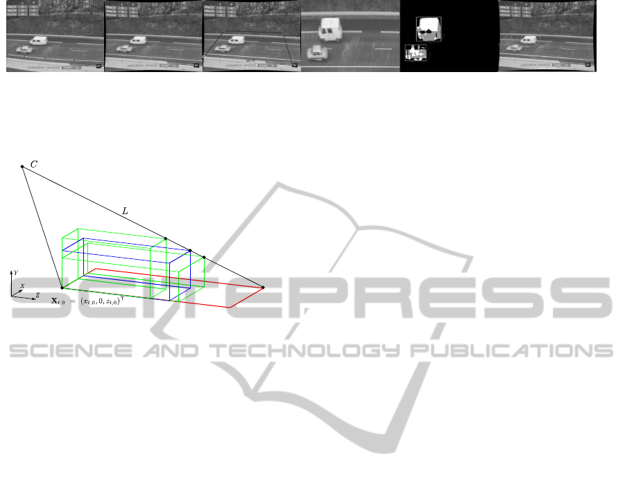
Figure 2: Pre-processing steps: (a) original image; (b) correction of lens distortion; (c) detection of orthogonal directions on
the plane; (d) rectified road plane; (e) detected 2D blobs using background segmentation; (f) 3D models after applying the
proposed method.
Figure 3: Projective ambiguity: a given 2D observation in
the OXZ plane (in red) of a true 3D cuboid (blue) may also
be the result of the projection of a family of cuboids (in
green) with respect to camera C.
might be any function from which it is easy to draw
samples. Typically it is chosen as a normal distribu-
tion, which is symmetric, i.e. q(x
j− 1
t
|x
j
t
) = q(x
j
t
|x
j− 1
t
)
and thus the terms depending on the proposal can be
removed from eq. 3.
Besides, it is a common practice to select a subset
of samples from the chain to reduce their correlation
and to discard a number of initial samples to reduce
the influence of initialization. Therefore, to obtain N
s
effective samples of the chain it is required to generate
a total number of samples N = B + cN
s
, where B is
the number of initial samples, and c is the number of
samples discarded per valid sample.
4 LIKELIHOOD FUNCTION
For each image, the observation is the current 2D sil-
houette of the vehicle projected into the rectified im-
age. Considering the cuboid-model of the vehicle,
and that the yaw angle is approximatedly zero we can
reproject a 3D ray from the far-most corner of the pro-
jected cuboid and the optical center.
There are infinite points on the ray that are pro-
jected in the same image point and therefore corre-
spond to a solution to the parameters of the cuboid, as
shown in Fig. 3. Nevertheless, there are a number of
constraints that bound the solution to a segment of the
ray: positive and minimum height, width and length.
Therefore, the likelihood function must be any
function that fosters volume hypotheses near the re-
projection ray. For the sake of simplicity, we choose a
normal distribution on the point-line distance. The co-
variance of the distribution expresses our confidence
about the measurement of the 2D silhouette and the
calibration information. The likelihood function can
be written as
p(z
t
|x
t
) ∝ exp

(y
t
− x
t
)
⊤
S
−1
(y
t
− x
t
)

(4)
where x
t
is a volume hypothesis, and y
t
is its projec-
tion onto the reprojection ray. The position of y
t
can
be computed from x
t
as the intersection of the ray and
a plane passing through x
t
and whose normal vector is
parallel to the ray. For this purpose we can represent
the ray as a Pl¨ucker matrix L
t
= ab
⊤
− ba
⊤
, where a
and b are two points of the line, e.g. the far-most point
of the 2D silhouette, and the optical center, respec-
tively. These two points are expressed in theWHL co-
ordinate system. Therefore, provided that we have the
calibration of the camera, we need a reference point
in the 2D silhouette. We have observed that the point
with less distortion is typically the closest point of the
quadrilateral to the optical center, whose coordinates
are X
t,0
= (x
t,0
,0,z
t,0
)
⊤
in the XYZ world coordinate
system. This way, any XYZ point can be transformed
into a WHL point as x
t
= R
0
X
t
− X
t,0
. Nevertheless,
the relative rotation between these systems can be ap-
proximated to the identity, since the vehicles typically
drive parallel to the OZ axis.
The plane is defined as π
t
= (n
⊤
t
,D
t
)
⊤
, where
n
t
= (n
x
,n
y
,n
z
)
⊤
is the normal to the ray L
t
, and
D
t
= −n
⊤
t
x
t
. Therefore, the projection of the point
on the ray can be computed as y
t
= L
t
π
t
.
5 PRIOR FUNCTIONS
The information about the volume of the vehicle can
be encoded as the product of two functions, each one
modeling two independent sources of information:
p(x
t
|x
t−1
,M ) = p(x
t
|x
t−1
)p(x
t
|M ) (5)
where p(x
t
|x
t−1
) represents the dynamic model of the
system. In our case, we will assume that a vehicle is
REAL-TIME 3D MODELING OF VEHICLES IN LOW-COST MONOCAMERA SYSTEMS
461

Figure 4: Projection of vehicle prior models into the ray L.
For a better visualization, each p(x
t
,x
m
) is shown as a point
in WHL and a contour slice parallel to OHL.
a non-deformable rigid object, such that it does not
vary its dimensions through time, and thus
p(x
t
|x
t−1
) ∝ exp

(x
t
− x
t−1
)
⊤
(x
t
− x
t−1
)

(6)
The second term of eq. (5), p(x
t
|M ), contains the
information that we have about typical configurations
of vehicle dimensions, i.e. typical proportions of ve-
hicles according to a number of models, such as truck,
motorcycle, car, etc. Let us represent this informa-
tion as a set of clusters that can be parameterized as
a mixture of normal distributions in the WHL space:
M = {x
m
}
M
m=1
. Therefore,
p(x
t
|M ) =
M
∑
m=1
p(x
t
,x
m
) (7)
where x
m
= (W
m
,H
m
,L
m
)
⊤
and
p(x
t
,x
m
) ∝ exp

(x
t
− x
m
)
⊤
S
−1
m
(x
t
− x
m
)

(8)
and S
m
= diag{σ
2
w
,σ
2
h
,σ
2
l
} is the covariance matrix of
model m.
Table 1 exemplifies a set of vehicle models. The
gaussian model ensures that the vehicle models are
not rigid nor fixed, in contrast with typical wireframe
models, and thus enhances the flexibility of prior in-
formation. For instance, trucks can be modeled as a
3D gaussian centered at (2.0,2.5,7) with high vari-
ance values, since trucks may vary significantly in
length or height.
6 ALGORITHM COMPLEXITY
REDUCTION
Once we have defined the prior and observation mod-
els, the complete expression of the MH acceptance
ratio is given by:
α =
p(z
t
|x
j
t
)
p(z
t
|x
j−1
t
)
∑
N
s
i=1
p(x
j
t
|x
i
t−1
)
∑
N
s
i=1
p(x
j−1
t
|x
i
t−1
)
∑
M
m=1
p(x
j
t
,x
m
)
∑
M
m=1
p(x
j−1
t
,x
m
)
(9)
Table 1: Example configuration of vehicle models.
Vehicle type W
m
H
m
L
m
σ
w
σ
h
σ
l
Car 1.6 1.5 4 0.1 0.1 0.2
Motorbike 1.6 1.5 2 0.1 0.1 0.2
Truck 2.0 2.5 7 0.2 0.3 1.0
Trailer 1.6 1.5 7 0.1 0.1 2.0
Bus 2.0 2.5 10 0.2 0.3 1.0
By drawing N
s
effective samples using the MH al-
gorithm we have the approximation of the posterior
distribution as in eq. (2). Hence, we can compute
point-estimates of the state vector x
t
and thus estimate
the volume of the 3D cuboid at each time instant. For
instance we can use the sample mean as the simplest
statistic, which is valid enough since the posterior dis-
tribution can be assumed to be unimodal.
Nevertheless, the generation of the Markov chain
implies a significant amount of computations, since
the computational complexity is O(NN
s
). The reason
is that for each proposed sample x
j
t
, the complete set
of previous samples {x
i
t−1
}
N
s
i=1
has to be evaluated to
compute the acceptance ratio.
To reduce to linear time operation, i.e. O(N), we
can instead select a single previous sample, x
∗
t−1
, from
the set. Khan et al. (Khan et al., 2005) propose to
select a random sample from the set, although we
have observed much better performance selecting the
point-estimate of the previous time instant. The ac-
ceptance ratio expression is then simplified to:
α =
p(z
t
|x
j
t
)
p(z
t
|x
j− 1
t
)
p(x
j
t
|x
∗
t−1
)
p(x
j− 1
t
|x
∗
t−1
)
∑
M
m=1
p(x
j
t
,x
m
)
∑
M
m=1
p(x
j− 1
t
,x
m
)
(10)
Regarding the specific nature of our problem, an
additional great reduction of the complexity of the
sampling step can be achieved if we force the sam-
ples to belong to the ray defined by the likelihood
model. This is equivalent to reduce the problem to a
one-dimensional search on the ray. On the one hand,
the proposal density can be now defined as a one-
dimensional normal distribution that draw samples on
the ray, as well as the dynamic model. Therefore, the
samples are now drawn based on the simplified ex-
pression of the acceptance ratio:
α =
p(x
j
t
|x
∗
t−1
)
p(x
j− 1
t
|x
∗
t−1
)
∑
M
m=1
p(x
j
t
,x
m
)
∑
M
m=1
p(x
j− 1
t
,x
m
)
(11)
subject to x
j
t
∈ L
t
.
The implementation of the algorithm can be as
well simplified if the state space is reduced to a dis-
crete number of states, namely {y
m
}
M
m=1
, i.e. the pro-
jections of the vehicle models on the observed ray.
VISAPP 2011 - International Conference on Computer Vision Theory and Applications
462

0
0,2
0,4
0,6
0,8
1
1,2
1 2 3 4 5 6 7 8 9 10 11
width error (m)
frames frames
0
1
2
3
4
5
6
1 2 3 4 5 6 7 8 9 10 11
length error (m)
2D - TRUCK
2D - CAR
3D - TRUCK
3D - CAR
(a) (b) (c) (d)
0
0,5
1
1,5
2
2,5
3
3,5
4
4,5
1 2 3 4 5 6 7 8
width error (m)
frames
0
0,2
0,4
0,6
0,8
1
1,2
1,4
1,6
1 2 3 4 5 6 7 8
length error (m)
2D - TRUCK
2D - CAR
3D - TRUCK
3D - CAR
frames
(e) (f) (g) (h)
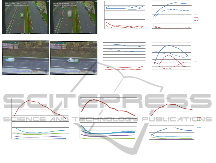
Figure 5: Examples of the error of the 2D and 3D methods for different perspectives and type of vehicles.
0
200
400
600
800
1000
1200
1400
1 2 3 4 5 6 7 8 9 10 11 12
0
100
200
300
400
500
600
700
800
900
1000
1 2 3 4 5 6 7 8 9 10 11 12 13 14
0
200
400
600
800
1000
1200
1 2 3 4 5 6 7 8 9 10 11
Car
Moto
Bus
Truck
Trailer
Mahalanobis distance
Figure 6: Mahalanobis distance for all the defined classes for three example sequences of a car, a bus and a truck.
Under this assumption, the algorithm computes the
posterior probability of each y
t,m
= L
t
π as propor-
tional to p(y
t,m
|y
∗
t−1
)p(y
t,m
,x
m
), and determines the
MAP point-estimate of p(x
t
|Z
t
) as the most likely
projection y
t,m
.
7 RESULTS
The proposed system overcomes the problems of 2D
strategies that aim to measure the dimensions of the
vehicles for classification purposes in perspective im-
ages. Fig. 5 shows some examples of the error com-
mitted by the proposed 3D estimation method and
the base 2D estimation strategy when computing the
width and length of a vehicle with known dimensions.
As shown, the perspective distortion causes that the
2D strategies incurr in severe estimation errors. For
instance, the images of the upper row of Fig. 5 de-
pict a situation in which the perspective of the cam-
era makes that 2D estimation of the length of the ve-
hicle are greatly incorrect, while the estimation ob-
tained by the proposed 3D module dramatically re-
duces the error. Analougously, the bottom row of Fig.
5 shows a case where the perspective affects mostly
the 2D estimation of the width of vehicles, while the
proposed method again achieves great reductions of
measurement error. As a consequence, the proposed
method helps to improve the reliability of a system
that aims to classify vehicles according to their di-
mensions, which is in turn quite typical in tolling ap-
plications.
Finally, we exemplify the classification quality of
our approach in Fig. 6, which corresponds to three
example sequences of a car, a bus, and a truck (with
typical dimensions). This figure shows the values of
the Mahalanobis distance of each model x
m
with re-
spect to their projections into the ray L. The classifica-
tion is correct as the “car”, “bus” and “truck” classes
obtain that lowest error along their corresponding se-
quences. As far as the instantaneous estimations are
coherent from one frame to another, the application of
the motion prior strengthens the classification.
In order to evaluate the performance of the vehi-
cle classification, we have tested the proposed solu-
tion for a set of videos of different roads and perspec-
tives, with an aggregateduration of more than 5 hours.
The total number of detected vehicles in the video se-
quence is 2551/2585 (98.7%). The target application
required the classification of vehicles into two broad
REAL-TIME 3D MODELING OF VEHICLES IN LOW-COST MONOCAMERA SYSTEMS
463

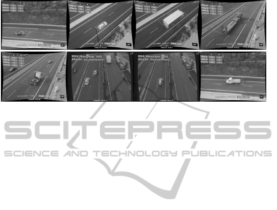
Figure 7: Example results of 3D vehicle modeling, including different size vehicles and type of perspectives.
categories: light and heavy. Considering the detected
vehicles, the system correctly classified 2214/2248
light vehicles, and 337/337 heavy vehicles according
to their volume. Some example images of the render-
ization of the estimated 3D model are shown in Fig. 7.
As shown, in most situations, the cuboid fits correctly
the volume occupied by the vehicles (with some un-
accuracy due to insufficient perpsective distortion or
excessively long vehicles), and thus allow to classify
vehicles in the required categories.
8 CONCLUSIONS
This paper introduces a real-time method to augment
2D vehicle detections into 3D volume estimations by
using prior vehicle models and projective constraints.
The solution is described as a MCMC-based MAP
method, on which several assumptions and simplifi-
cations are applied in order to dramatically reduce the
complexity of the algorithm. Tests have shown excel-
lent classification results under different perspectives
in the presence of vehicles with heavily varied dimen-
sions and shapes.
ACKNOWLEDGEMENTS
The authors would like to thank the Basque Govern-
ment for the funding provided through the ETORGAI
strategic project iToll.
REFERENCES
Arulampalam, M. S., Maskell, S., Gordon, N., and Clapp,
T. (2002). A tutorial on particle filters for on-
line nonlinear/non-gaussian bayesian tracking. IEEE
Transactions on Signal Processing, 50(2):174–188.
Barder, F. and Chateau, T. (2008). MCMC particle filter
for real-time visual tracking of vehicles. In IEEE In-
ternational Conference on Intelligent Transportation
Systems, pages 539–544.
Buch, N., Orwell, J., and Velastin, S. A. (2010). Urban road
user detection and classification using 3d wire frame
models. IET Computer Vision Journal, 4(2):105–116.
Haag, M. and Nagel, H.-H. (2000). Incremental recogni-
tion of traffic situations from video image sequences.
Image and Vision Computing, 18:137–153.
Isard, M. and Blake, A. (1998). CONDENSATION– con-
ditional density propagation for visual tracking. Inter-
national Journal of Computer Vision, 29(1):5–28.
Khan, Z., Balch, T., and Dellaert, F. (2005). MCMC-based
particle filtering for tracking a variable number of in-
teracting targets. IEEE Transactions on Pattern Anal-
ysis and Machine Intelligence, 27(11):1805–1819.
Kim, K., Chalidabhongse, T. H., Harwood, D., and Davis,
L. (2005). Real-time foreground-background segmen-
tation using codebook model. Real-time Imaging,
11(3):167–256.
Pang, C., Lam, W., and Yung, N. (2007). A method for
vehicle count in the presence of multiple occlusions
in traffic images. IEEE Transactions on Intelligent
Transportation Systems, 8(3):441–459.
VISAPP 2011 - International Conference on Computer Vision Theory and Applications
464