
ROBUST MOBILE OBJECT TRACKING BASED ON MULTIPLE
FEATURE SIMILARITY AND TRAJECTORY FILTERING
Duc Phu Chau, Franc¸ois Bremond, Monique Thonnat and Etienne Corvee
Pulsar team, INRIA Sophia Antipolis - M´editerran´ee, Sophia Antipolis, France
Keywords:
Tracking algorithm, Trajectory filter, Global tracker, Tracking evaluation.
Abstract:
This paper presents a new algorithm to track mobile objects in different scene conditions. The main idea
of the proposed tracker includes estimation, multi-features similarity measures and trajectory filtering. A
feature set (distance, area, shape ratio, color histogram) is defined for each tracked object to search for the best
matching object. Its best matching object and its state estimated by the Kalman filter are combined to update
position and size of the tracked object. However, the mobile object trajectories are usually fragmented because
of occlusions and misdetections. Therefore, we also propose a trajectory filtering, named global tracker,
aims at removing the noisy trajectories and fusing the fragmented trajectories belonging to a same mobile
object. The method has been tested with five videos of different scene conditions. Three of them are provided
by the ETISEO benchmarking project (http://www-sop.inria.fr/orion/ETISEO) in which the proposed tracker
performance has been compared with other seven tracking algorithms. The advantages of our approach over
the existing state of the art ones are: (i) no prior knowledge information is required (e.g. no calibration and no
contextual models are needed), (ii) the tracker is more reliable by combining multiple feature similarities, (iii)
the tracker can perform in different scene conditions: single/several mobile objects, weak/strong illumination,
indoor/outdoor scenes, (iv) a trajectory filtering is defined and applied to improve the tracker performance, (v)
the tracker performance outperforms many algorithms of the state of the art.
1 INTRODUCTION
Many different approaches have been proposed to
track the motion of mobile objects in video (A. Yil-
maz et al., 2006). However the tracking algorithm
performance is always dependant on scene conditions
such as illumination, occlusion frequence, movement
complexity level. Some researches aim at improving
the tracking quality by extracting the scene informa-
tion such as: directions of paths, interesting zones.
These elements can help the system to give a better
prediction and decision on object trajectories. For
example (D. Makris and T. Ellis, 2005) have pre-
sented a method to model the paths in scenes based
on detected trajectories. The system uses an unsu-
pervised machine learning technique to compute tra-
jectory clustering. A graph is automatically built to
represent the path structure resulting from learning
process. In (D. P. Chau et al., 2009a), the authors
have proposed a global tracker to repair lost trajecto-
ries. The system learns automatically the “lost zone”
where the tracked objects usually lose their trajecto-
ries and “found zone” where the tracked objects usu-
ally reappear. The system also takes complete trajec-
tories to learn the common scene paths composed by
<entrance zone, lost zone, found zone>. The learnt
paths are then used to fuse the lost trajectories. This
algorithm needs a 3D calibration environment and
also a 3D person model as the inputs. These two pa-
pers get some good results but both require an off-line
machine learning process to create rules for improv-
ing the tracking quality.
In order to solve the given problems in mobile
object tracking, we propose in this paper a multi-
ple feature tracker combining with a global tracking.
We use first the Kalman filter to predict positions of
tracked objects. However, this filter is only an esti-
mator for linear movements while the object move-
ments in surveillance videos are usually complex. A
poor lighting condition of scene also influences to the
tracking quality. Therefore, in this paper we propose
to use different features to obtain more correct match-
ing links between objects in a given time window. We
also define a global tracker which does not require
3D environment calibration or off-line learning to im-
prove tracking quality.
The rest of paper is organized as follows: The next
section presents in detail the tracking process. Section
569
Phu Chau D., Bremond F., Thonnat M. and Corvee E..
ROBUST MOBILE OBJECT TRACKING BASED ON MULTIPLE FEATURE SIMILARITY AND TRAJECTORY FILTERING.
DOI: 10.5220/0003317205690574
In Proceedings of the International Conference on Computer Vision Theory and Applications (VISAPP-2011), pages 569-574
ISBN: 978-989-8425-47-8
Copyright
c
2011 SCITEPRESS (Science and Technology Publications, Lda.)

3 describes a global tracking algorithm which aims at
filtering out noisy trajectories and fusing fragmented
trajectories. This section also presents when a tracked
object ends its trajectory. Section 4 shows in detail the
results of the experimentation and validation. A con-
clusion is given in the last section as well as future
work.
2 TRACKING ALGORITHM
The proposed tracker takes as its input a bounding
box list of detected objects at each frame. Pixel val-
ues inside these bounding boxes are also required to
compute color metric. A tracked object at frame t is
represented by a state s = [x,y,l, h] where (x, y) is
center position, l is width and h is height of its 2D
object bounding box at frame t. In the tracking pro-
cess, we follow three steps of the Kalman filter: es-
timation, measurement and correction. However our
contribution focus on the measurement step. The es-
timation step is first performed to estimate the new
state of a tracked object in the current frame. The
measurement step is then performed to search for the
best detected object similar to each tracked object in
the previous frames. The state of the found object
refers to as “measured state”. The correction step is
finally performed to compute the “corrected state” of
mobile object resulting from the “estimated state” and
the “measured state”. This state is considered as the
official state of the considered tracked object in the
current frame. For each detected object which does
not match with any tracked object, a new tracked ob-
ject with the same position and size will be created.
2.1 Estimation of Position and Size
For each tracked object in the previous frame, the
Kalman filter is used to estimate the new state of the
object in the current frame. The Kalman filter is com-
posed of a set of recursive equations used to model
and evaluate object linear movement. Let s
+
t−1
be the
corrected state at instant t − 1, the estimated state at
time t, denoted s
−
t
, is computed as follows:
s
−
t
= Φs
+
t−1
(1)
where Φ is the state transition matrix of n x n where n
is the considered feature number (n = 4 in our case).
Note that in practice Φ might change with each time
step, but here we assume it is constant. One of the
drawbacks of the Kalman filter is the restrictive as-
sumption of Gaussian posterior density functions at
every time step, as many tracking problems involve
non-linear movement. In order to overcome this limi-
tation, we give a weight value to determine the relia-
bility of estimation computation and also of measure-
ment (see section 2.3 for details).
2.2 Measurement
This is our main contribution in the tracking process.
For each tracked object in the previous frame, the goal
of this step is to search for the best matched object
in the current frame. In tracking problem, the exe-
cution time of tracking algorithm is very important
to assure a real time system. Therefore, in this pa-
per we propose to use a set of four features: distance,
shape ratio, area and color histogram to compute the
similarity between two objects. The computation of
all of these features are not time consuming and the
proposed tracker can thus be executed in real time.
Because all measurements are computed in the 2D
space, our proposed method does not require scene
calibration information. For each feature i (i = 1..4),
we define a local similarity LS
i
in the interval [0, 1]
to quantify the object similarity of the feature i. A
global similarity is defined as a combination of these
local similarities. The detected object with the high-
est global similarity will be chosen for the correction
step.
2.2.1 Distance Similarity
The distance between two objects is computed as the
distance between the two corresponding object posi-
tions. Let D
max
be the possible maximal displacement
of mobile object for 1 frame in video and d be the
distance of two considered objects in two consecutive
frames, we define a local similarity LS
1
between these
two objects using distance feature as follows:
LS
1
= max(0, 1− d/(D
max
∗ m)) (2)
where m is the temporal difference (frame unity) of
the two considered objects.
In a 3D calibration environment, a value of D
max
can be set for the whole scene. However, this value
should not be unique in a 2D scene. This threshold
will change according to the distance between con-
sidered objects and the camera position. The nearer
object to the camera, the larger its displacement is.
In order to overcome this limitation, we set the D
max
value to the length half of bounding box diagonal of
the considered tracked object.
2.2.2 Area Similarity
The area of an object i is calculated by W
i
H
i
where
W
i
and H
i
are the 2D width and height of the object
VISAPP 2011 - International Conference on Computer Vision Theory and Applications
570

respectively. A local similarity LS
2
between two areas
of objects i and j is defined by:
LS
2
=
min(W
i
H
i
, W
j
H
j
)
max(W
i
H
i
, W
j
H
j
)
(3)
2.2.3 Shape Ratio Similarity
The shape ratio of an object i is calculated by W
i
/H
i
(whereW
i
and H
i
are defined in section 2.2.2). A local
similarity LS
3
between two shape ratios of objects i
and j is defined as follows:
LS
3
=
min(W
i
/H
i
, W
j
/H
j
)
max(W
i
/H
i
, W
j
/H
j
)
(4)
2.2.4 Color Histogram Similarity
In this work, the color histogram of a mobile object
is defined as a histogram of pixel number inside its
bounding box. Other color features (e.g. MSER) can
be used but this one has given satisfying results. We
define a local similarity LS
4
between two objects i and
j for color feature as follows:
LS
4
=
∑
n
k=1
rate
k
n
(5)
where n is a parameter representing the number of his-
togram bins, n = 1..768 (the value 768 is the result of
product 256 x 3) and rate
k
is computed as follows:
rate
k
=
min(H
i
(k),H
j
(k))
max(H
i
(k),H
j
(k))
(6)
H
i
(k) and H
j
(k) are successively the number of pixels
of object i, j at bin k. There are some different ways
to compute the difference between two histograms, in
this work we choose the ratio computation for each
histogram bin to obtain a value rate
k
normalised in
the interval [0, 1]. Consequently the LS
4
value also
varies in this interval.
2.2.5 Global Similarity
A detected object compared to previous frames can
have some size variations because of detection er-
rors or some color variations by illumination changes,
but its maximum speed cannot exceed a determined
value. Therefore in our work, the global similarity
value takes into account a priority of distance feature
compared to other features to decrease the number of
false object matching links.
GS =
∑
4
i=1
w
i
LS
i
∑
4
j=1
w
j
if LS
1
> 0
0 otherwise
(7)
where GS is the global similarity; w
i
is the weight (i.e.
reliability) of feature i and LS
i
is the local similarity of
feature i. The detected object with the highest global
similarity value GS will be chosen as the matched ob-
ject if:
GS ≥ T
1
(8)
where T
1
is a predefined threshold. Higher the value
of T
1
is set, more correct the matching links are es-
tablished, but a too high value of T
1
can make lose
the matching links in some complex environment(e.g.
poor lighting condition, occlusion). The state of this
object (including its position and its bounding box
size) is called “measured state”. At a time instant t,
if a tracked object cannot find its matched object, the
measured state MS
t
is set to 0. In the experimenta-
tion of this work, we suppose that all feature weight
w
i
have the same values.
2.3 Correction
Thanks to the estimated and measured states, we can
update the position and size of tracked object by com-
puting the corrected state as follows:
CS
t
=
wMS
t
+ (1− w)ES
t
if MS
t
6= 0
MS
t−1
otherwise
(9)
where CS
t
, MS
t
, ES
t
are the corrected state, measured
state and estimated state of the tracked object at time
instant t respectively; w is the weight of measurement
state. If the measured state is not found, the corrected
state will be set equal to the corrected state in the pre-
vious frame. While the estimated state is only result
of a simple linear estimator, the measurement step is
fulfilled by considering four different features. We
thus set a high value to w (w = 0.7) in our experimen-
tation.
3 GLOBAL TRACKING
ALGORITHM
Global tracking aims at fusing the fragmented trajec-
tories belonging to a same mobile object and remov-
ing the noisy trajectories. As mentioned in section
2.3, if a tracked object cannot find the correspond-
ing detected object, his corrected state will be set to
the current corrected state. The object then turns into
a “waiting state”. This tracked object goes out of
“waiting state” when it finds its matched object. A
tracked object can turn into and go out of “waiting
state” many times during its life. This waiting step
allows us to let a non-updated tracks live for some
ROBUST MOBILE OBJECT TRACKING BASED ON MULTIPLE FEATURE SIMILARITY AND TRAJECTORY
FILTERING
571

frames when no correspondence is found. The sys-
tem can so track completely object motion even when
the object is not sometime detected or is detected in-
correctly. This prevents the mobile object trajectories
from being fragmented. However, the “waiting state”
can cause an error when the correspondingmobile ob-
ject goes out of the scene definitively. Therefore, we
propose a rule to decide the moment when a tracked
object ends its life and also to avoid maintaining for
too long the “waiting state”. A more reliable tracked
object will be kept longer in the “waiting state”. In
our work, the tracked object reliability is directly pro-
portional to number of times this object finds matched
objects. The greater number of matched objects, the
greater tracked object reliability is. Let Id of a frame
be the order of this frame in the processed video se-
quence, a tracked object ends if:
F
l
< F
c
− min(N
r
,T
2
) (10)
where F
l
is the latest frame Id where this tracked ob-
ject finds matched object (i.e. the frame Id before en-
tering the “waiting state”), F
c
is the current frame Id,
N
r
is the number of frames in which this tracked ob-
ject was matched with a detected object, T
2
is a pa-
rameter to determine the number of frames for which
the “waiting state” of a tracked object cannot exceed.
With this calculation method, a tracked object that
finds a greater number of matched objects is kept in
the “waiting state” for a longer time but its “waiting
state” time never exceed T
2
. Higher the value of T
2
is set, higher the probability of finding lost objects is,
but this can decrease the correctness of the fusion pro-
cess.
We also propose a set of rules to detect the noisy
trajectories. The noise usually appears when wrong
detection or misclassification (e.g. due to low image
quality) occurs. A static object or some image regions
can be detected as a mobile object. However, a noise
usually only appears in few frames or does not dis-
place really (around a fixed position). We thus pro-
pose to use temporal and spatial filters to remove it. A
trajectory is composed of objects throughout time, so
it is unreliable if it cannot contain enough objects and
usually lives in the “waiting state”. Therefore we de-
fine a temporal threshold when a “waiting state” time
is greater, the corresponding trajectory is considered
as noise. Also, if a new trajectory appears, the system
cannot determine immediately whether it is noise or
not. The global tracker has enough information to fil-
ter out it only after some frames since its appearance
moment. Consequently, a trajectory that satisfies one
of the following conditions, is considered as noise:
T < T
3
(11)
(d
max
< T
4
) and (T ≥ T
3
) (12)
(
T
w
T
≥ T
5
) and (T ≥ T
3
) (13)
where T is time length (number of frames) of the
considered trajectory (“waiting state” time included);
d
max
is the maximum spatial length of this trajectory;
T
w
is the total time of “waiting state” during the life of
the considered trajectory; T
3
, T
4
and T
5
are the prede-
fined thresholds. While T
4
is a spatial filter threshold,
T
3
and T
5
can be considered as temporal filter thresh-
olds to remove noisy trajectories. The condition (11)
is only examined for the trajectories which end their
life according to equation (10).
4 EXPERIMENTATION
AND VALIDATION
We can classify the tracker evaluation methods by
two principal approaches: off-line evaluation using
ground truth data (C. J. Needham and R. D. Boyle,
2003) and on-line evaluation without ground truth
data (D. P. Chau et al., 2009b). In order to be able
to compare our tracker performance with the other
ones, we decide to use the tracking evaluation met-
rics defined in ETISEO benchmarking project (A.
T. Nghiem et al., 2007) which comes from the first
approach. The first tracking evaluation metric M
1
,
which is the “tracking time” metric measures the
percentage of time during which a reference object
(ground truth data) is tracked. The second metric
M
2
“object ID persistence” computes throughout time
how many tracked objects are associated with one ref-
erence object. The third metric M
3
“object ID confu-
sion” computes the number of reference object IDs
per tracked object. These metrics must be used to-
gether to obtain a complete tracker evaluation. There-
fore, we also define a tracking metric M taking the
average value of these three tracking metrics. All of
the four metric valuesare defined in the interval [0, 1].
The higher the metric value is, the better the tracking
algorithm performance gets.
In this experimentation, we use the people de-
tection algorithm based on HOG descriptor of the
OpenCV library (http://opencv.willowgarage.com/
wiki/). Therefore we focus the experimentation on
the sequences containing people movements. How-
ever the principle of the proposed tracking algorithm
is not dependent on tracked object type.
We have tested our tracker with five video se-
quences. The first three videos are selected from
ETISEO data in order to compare the proposed
tracker performance with that from other teams. The
last two videos are extracted from different projects
so that the proposed tracker can be tested with more
VISAPP 2011 - International Conference on Computer Vision Theory and Applications
572
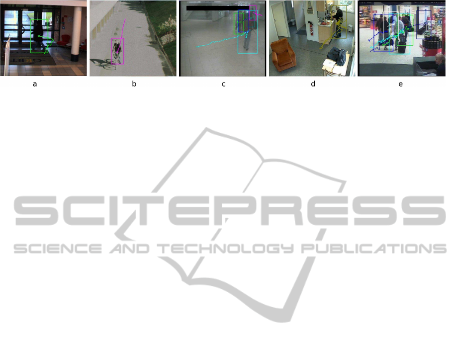
Figure 1: Illustration of tested videos: a) ETI-VS1-BE-18-C4 b) ETI-VS1-RD-16-C4 c) ETI-VS1-MO-7-C1 d) Gerhome
e)
˜
TRECVid. The colors represent the bounding boxes and trajectories of tracked people.
scene conditions. All of these five videos are tested
with the following parameter values: n = 96 bins (for-
mula (5)), T
1
= 0.8 (formula (8)), T
2
= 20 frames (for-
mula (10)), T
3
= 20 frames (formula (11)), T
4
= 5 pix-
els (formula (12)) and T
5
= 40% (formula (13)).
The first tested ETISEO video shows a building
entrance, denoted ETI-VS1-BE-18-C4. In this se-
quence, there is only one person moving, but the il-
lumination and contrast level are low (see image a of
figure 1). The second ETISEO video shows a road
with strong illumination, denoted ETI-VS1-RD-16-
C4 (see image b of figure 1). There are walker, bi-
cyclists, car moving on the road. The third video
shows an underground station denoted ETI-VS1-MO-
7-C1 where there are many complex people move-
ments (see image c of figure 1). The illumination and
contrast in this sequence are very bad.
In this experimentation, tracker results from seven
different teams in ETISEO have been presented: 1,
8, 11, 12, 17, 22, 23. Table 1 presents performance
results of our tracker and of the ones of seven teams
on three ETISEO sequences. Although each tested
video has its proper complex, the tracking evaluation
metrics of the proposed tracker get the highest values
in most cases compared to other teams. In the second
video, the tracking time of our tracker is low (M
1
=
0.36) because as mentioned above, we only use the
people detector and so system usually fails to detect
cars.
The fourth video sequence has been provided by
the Gerhome project (see image d of figure 1). The
objective of this project is to enhance autonomy of the
elderly people at home by using intelligent technolo-
gies for house automation. In this sequence, there is
only one person moving but the video length is quite
long (13 minutes 40 seconds). We can find tracking
results in the second column of table 2. Although the
sequence length is quite long, the proposed tracker
can follow person movement for most of the time,
from frame 1 to frame 8807 (M
1
= 0.86). After that,
there are four moments when the detection algorithm
cannot detect the person in an interval over 20 frames
(over the value of T
2
). Therefore the value of metric
M
2
for this video sequence is only equal to 0.2.
The last tested sequence concerns the movements
of people in an airport. This sequence is provided
by TREC Video Retrieval Evaluation (TRECVid) (A.
Smeaton et al., 2006). The people tracking in this se-
quence is a very hard task because there are always a
great number of movements in the scene and occlu-
sions usually happen (see image e of figure 1). De-
spite these difficulties, the proposed tracker obtains
high values for all three tracking evaluation metrics:
M
1
= 0.71, M
2
= 0.90 and M
3
= 0.85 (see the third
column of table 2).
The average processing speed of the proposed
tracking algorithm for all considered sequences is
very high. In the most complicated sequence where
there are many crowds (TRECVid sequence), this
value is equal to 20 f ps. In the other video se-
quences, the average processing speed of the tracking
task is greater than 50 f ps. This helps whole track-
ing framework (including video acquisition, detection
and tracking tasks) can become a real time system.
5 CONCLUSIONS
Although many researches aim at resolving the prob-
lems given by tracking process such as misdetection,
occlusion, there is still not a robust tracker which can
well perform in different scene conditions. This pa-
per has presented a tracking algorithm which is com-
bined with a global tracker to increase the robustness
of the tracking process. The proposed approach has
been tested and validated on fivereal video sequences.
The experimentation results show that the proposed
tracker can obtain good tracking results in many dif-
ferent scenes although each tested scene has its proper
complexity. Our tracker also gets the best perfor-
mances in the experimented ETISEO videos com-
pared to other tracker evaluated in this project. The
average processing speed of the proposed tracking al-
gorithm is high. However, some drawbacks still exist
in this approach: the used features are simple, more
complex features (e.g. color covariance) are needed
ROBUST MOBILE OBJECT TRACKING BASED ON MULTIPLE FEATURE SIMILARITY AND TRAJECTORY
FILTERING
573

Table 1: Summary of tracking results for ETISEO videos.
N: video frame number, F: video frame rate, s : average
processing speed of the tracking task ( f rames/second) (not
taking into account the detection process). The highest val-
ues are printed bold.
ETI-VS1-
BE-18-C4
ETI-VS1-
RD-16-C4
ETI-VS1-
MO-7-C1
N 1108 1315 2282
F 25 f ps 16 f ps 25 f ps
M
1
0.64 0.36 0.87
Proposed M
2
1 1 0.92
tracker M
3
1 1 1
M 0.88 0.79 0.93
s 292 f ps 641 f ps 84 f ps
M
1
0.48 0.44 0.77
Team M
2
0.80 0.81 0.78
1 M
3
0.83 0.61 1
M 0.70 0.62 0.85
M
1
0.49 0.32 0.58
Team M
2
0.80 0.62 0.39
8 M
3
0.77 0.52 1
M 0.69 0.49 0.66
M
1
0.56 0.53 0.75
Team M
2
0.71 0.94 0.61
11 M
3
0.77 0.81 0.75
M 0.68 0.76 0.70
M
1
0.19 0.40 0.58
Team M
2
1 1 0.39
12 M
3
0.33 0.83 1
M 0.51 0.74 0.91
M
1
0.17 0.35 0.80
Team M
2
0.61 0.81 0.57
17 M
3
0.80 0.66 0.57
M 0.53 0.61 0.65
M
1
0.26 0.36 0.78
Team M
2
0.35 0.43 0.36
22 M
3
0.33 0.20 0.54
M 0.31 0.33 0.56
M
1
0.05 0.03 0.05
Team M
2
0.46 0.73 0.61
23 M
3
0.39 0.23 0.42
M 0.30 0.33 0.36
to obtain the more reliable matching links between
objects. We also propose in future work an on-line
automatic learning of the detected trajectories to im-
prove the global tracker quality.
ACKNOWLEDGEMENTS
This work is supported by The PACA region,
The General Council of Alpes Maritimes province,
France as well as The ViCoMo, Vanaheim, Video-Id,
Cofriend and Support projects.
Table 2: Tracking results for Gerhome and TRECVid
videos. s denotes the average processing speed of the track-
ing task (frames/second).
Gerhome TRECVid
Number of frames 10240 5000
Frame rate 12 f ps 25 f ps
M
1
0.86 0.71
M
2
0.20 0.90
M
3
1 0.85
M 0.69 0.82
s 58 f ps 20 f ps
REFERENCES
A. Smeaton, P. Over, and W. Kraaij (2006). Evaluation cam-
paigns and trecvid. In The MIR’06: The proceedings
of the ACM International Workshop on Multimedia In-
formation Retrieval.
A. T. Nghiem, F. Bremond, M. Thonnat, and V. Valentin.
(2007). Etiseo, performance evaluation for video
surveillance systems. In The IEEE International Con-
ference on Advanced Video and Signal based Surveil-
lance (AVSS), London, United Kingdom.
A. Yilmaz, O. Javed, and M. Shah (2006). Object track-
ing: A survey. The Journal ACM Computing Surveys
(CSUR).
C. J. Needham and R. D. Boyle (2003). Performance evalu-
ation metrics and statistics for positional tracker eval-
uation. In The International Conference on Computer
Vision Systems (ICVS), Graz, Austria.
D. Makris and T. Ellis (2005). Learning semantic scene
models from observing activity in visual surveillance.
In The IEEE Transactions on Systems, Man and Cy-
bernetics.
D. P. Chau, F. Bremond, E. Corvee, and M. Thonnat
(2009a). Repairing people trajectories based on point
clustering. In The International Conference on Com-
puter Vision Theory and Applications (VISAPP), Lis-
boa, Portugal.
D. P. Chau, F. Bremond, and M. Thonnat (2009b). Online
evaluation of tracking algorithm performance. In The
International Conference on Imaging for Crime De-
tection and Prevention (ICDP), London, United King-
dom.
VISAPP 2011 - International Conference on Computer Vision Theory and Applications
574
