
3D OBJECT CATEGORIZATION WITH PROBABILISTIC
CONTOUR MODELS
Gaussian Mixture Models for 3D Shape Representation
Kerstin P
¨
otsch and Axel Pinz
Inst. of El. Meas. and Measurement Sig. Proc., Graz University of Technology, Kopernikusgasse 24/IV, Graz, Austria
Keywords:
3D Object categorization, 3D Contour model, Gaussian mixture models.
Abstract:
We present a probabilistic framework for learning 3D contour-based category models represented by Gaus-
sian Mixture Models. This idea is motivated by the fact that even small sets of contour fragments can carry
enough information for a categorization by a human. Our approach represents an extension of 2D shape based
approaches towards 3D to obtain a pose-invariant 3D category model. We reconstruct 3D contour fragments
and generate what we call ‘3D contour clouds’ for specific objects. The contours are modeled by probability
densities, which are described by Gaussian Mixture Models. Thus, we obtain a probabilistic 3D contour de-
scription for each object. We introduce a similarity measure between two probability densities which is based
on the probability of intra-class deformations. We show that a probabilistic model allows for flexible modeling
of shape by local and global features. Our experimental results show that even with small inter-class difference
it is possible to learn one 3D Category Model against another category and thus demonstrate the feasibility of
3D contour-based categorization.
1 MOTIVATION AND IDEA
Shape features, especially contour features are chal-
lenging in computer vision for several reasons. The
research topics vary from 2D contour generation,
2D object recognition and categorization to 3D con-
tour reconstruction from multiview-stereo image se-
quences or 3D contour generation from 3D mod-
els. This paper deals with object categorization based
on 3D contour models, which we call ‘3D contour
clouds’. We represent these ‘3D contour clouds’ by
Mixture of Gaussian Models and we learn partitions
of probability density functions to achieve a 3D cate-
gory shape model.
In 2D, shape features play an important role for
object categorization. Contour features, e.g. silhou-
ette features as well as inner contours, have success-
fully been used in several recent categorization sys-
tems (Leordeanu et al., 2007), (Opelt et al., 2006),
(Shotton et al., 2008). These approaches are based
on fragments of contours (Opelt et al., 2006; Shot-
ton et al., 2008) or by simplifying them to a sparse
point representation (Leordeanu et al., 2007). In such
systems, 2D contour features are used to model the
shape of various object categories. Either, these cat-
egory models are learned in a 2D Implicit Shape
Model (ISM) (Leibe et al., 2004) manner, where an
object center is used as reference point to build in-
direct relations between pairs of contour fragments
and this ‘centroid’ (Opelt et al., 2006), (Shotton et al.,
2008), or they are learned using direct pairwise re-
lations between such contour fragments (Leordeanu
et al., 2007). The main disadvantage of these 2D
shape models is their view dependency because they
are quite sensitive to view/pose changes and conse-
quently, one model per significant aspect of a category
has to be learned independently to achieve robustness
to view and pose changes.
(a) (b)
Figure 1: (a) A horse, shown as a collection of 3D line seg-
ments (b).
2D object categorization building on 2D contour
models (Opelt et al., 2006; Shotton et al., 2008) re-
lies on the fact that contour fragments are sufficient to
259
Pötsch K. and Pinz A..
3D OBJECT CATEGORIZATION WITH PROBABILISTIC CONTOUR MODELS - Gaussian Mixture Models for 3D Shape Representation.
DOI: 10.5220/0003317402590270
In Proceedings of the International Conference on Computer Vision Theory and Applications (VISAPP-2011), pages 259-270
ISBN: 978-989-8425-47-8
Copyright
c
2011 SCITEPRESS (Science and Technology Publications, Lda.)

represent object shape (Lowe and Binford, 1983). By
looking at Figure 1(b), humans can easily identify the
object based on this simple collection of straight 3D
lines. We want to extend the idea of a 2D shape model
for categorization to 3D to obtain a pose-invariant 3D
category model. Therefore, we make use of the fol-
lowing principle:
Let us assume that we have a 3D model of an ob-
ject such as the horse in Figure 1(a). Such a horse
consists of several parts, e.g. head, legs, back, tail etc.
We can assume, that all these parts are in a spatial re-
lation to each other which can be described by proba-
bilities. Furthermore, if these parts are represented by
3D contour fragments, we can assume that these 3D
contour fragments are in a spatial relation and orienta-
tion to each other. So, each object can be described by
a small set of fragments having a specified orientation
and spatial relation to each other.
Our approach can then be summarized as follows:
We use probabilistic density functions for 3D shape
modeling. 3D contour fragments - 3D manifolds in
1D - are represented as Gaussian Mixture Models
(GMMs). These 3D contour fragments are recon-
structed from stereo image sequences, and build ‘3D
contour clouds’ for specific objects of a category. We
learn partitions of probability density functions us-
ing a random feature selection algorithm. The dis-
tance function for such partitions is based on pairwise
spatial relations and a similarity measure for mixture
components. In contrast to 2D based approaches we
build one single 3D model per category instead of one
2D model per significant view.
The contributions of this paper are
• 3D shape modeling by using GMMs for 3D con-
tour fragments, and
• Learning of a pose-invariant 3D Contour Cate-
gory Model consisting of partitions of probability
densities between two categories with small inter-
class difference.
2 STATE-OF-THE-ART
Based on the contributions of this paper, this section
is divided into three parts: 3D contour generation, 3D
shape modeling and matching, and Gaussian Mixture
Models for shape representation and matching.
The research on 3D contours (1D surface em-
bedded in 3D) so far concentrates on 3D curve re-
construction (Ebrahimnezhad and Ghassemian, 2007;
Park and Han, 2002; Fabbri and Kimia, 2010) or 3D
contour extraction from 3D surface models (DeCarlo
et al., 2003; DeCarlo and Rusinkiewicz, 2007; Ohtake
et al., 2004; Pauly et al., 2003). (Ebrahimnezhad and
Ghassemian, 2007) present a 3D contour reconstruc-
tion method based on the usage of a double stereo rig.
They describe a method for 3D reconstruction of ob-
ject curves from different views and motion estima-
tion based on these 3D curves. (Park and Han, 2002)
propose a method for Euclidean contour reconstruc-
tion including self-calibration. Unfortunately, this
contour matching algorithm is not applicable to our
image sequences. Recently, (Fabbri and Kimia, 2010)
presented an approach for multi-view stereo recon-
struction and calibration of curves. They concentrate
on the reconstruction of contour fragments assuming
that motion analysis can be obtained by other meth-
ods and their algorithm is mainly based on so called
view-stationary curves, e.g. shadows, sharp ridges,
reflectance curves. Therefore, it is well applicable
for aerial images, as they show in their results. 3D
contour extraction methods are manifold and differ
mainly in the type of the extracted contour/line frag-
ments, e.g. occluding contours, ridges (Ohtake et al.,
2004), suggestive contours (DeCarlo et al., 2003),
suggestive highlights and principal highlights (De-
Carlo and Rusinkiewicz, 2007). For a more detailed
literature overview we refer to the mentioned publica-
tions. As described in Appendix A, we use a method
where 3D contour fragments are reconstructed from
stereo image sequences. Our goal is to reconstruct
a qualitative ‘3D contour cloud’ representation rather
than precise 3D contours for the shape of a category,
which is not possible just based on stereo sequences.
There are many 3D shape matching approaches,
where a 3D shape is directly matched to a 3D model
database, such as the Princeton Shape Benchmark
(Shilane et al., 2004) and the ISDB (Gal et al.,
2007a). Point clouds, generated by laser range scan-
ners, by stereo vision, or by Structure-from-Motion
techniques, are probably the most obvious and sim-
plest way to represent 3D shape. Often, these point
clouds are converted to triangle meshes or polygonal
models. The research which has been done to an-
alyze, match and classify such models is extensive.
The shape representations vary from shape distribu-
tions (Gal et al., 2007b; Mahmoudi and Sapiro, 2009;
Ohbuchi et al., 2005; Osada et al., 2002) to symmetry
descriptors (Kazhdan et al., 2004) or Skeletal Graphs
(Sundar et al., 2003). In (Iyer et al., 2005; Tan-
gelder and Veltkamp, 2007) several shape represen-
tation methods are discussed. To our knowledge, the
method suggested in this paper is the first to demon-
strate learning on the basis of 3D contour fragments.
Gaussian Mixture Models often have been used
for shape modeling and shape matching, especially
for point set registration (Cootes, 1999; Wang et al.,
VISAPP 2011 - International Conference on Computer Vision Theory and Applications
260

2008; Peter and Rangarajan, 2009; Jian and Vemuri,
2005). Most of such methods take into account
the whole Gaussian Mixture Models shape match-
ing by defining or approximating information theo-
retic divergences on these mixtures. In contrast, we
learn partitions of Mixture of Gaussians by consid-
ering pairwise relations between probability density
functions and a similarity measure between densities
based on the principal eigenvector.
3 3D MIXTURE OF GAUSSIAN
CONTOUR MODEL
Modeling 3D contour fragments by probability den-
sity functions has several advantages. In particular,
noise, outliers and deformations can be handled in
a simple, natural way. Our algorithm is applicable
to all kind of 3D contour fragments which describe
the shape of a category. As mentioned in Section 2,
there are many possibilities to generate 3D contour
fragments. For the experiments of this paper, we re-
construct 3D contour fragments which build ‘3D con-
tour clouds’ from stereo image sequences of several
objects. The ‘3D contour cloud’ generation is not
the main contribution of this paper, and therefore, it
is covered in Appendix A. An example ‘3D contour
cloud’ of a horse is shown in Figure 2.
Figure 2: ‘3D contour cloud’ of a horse. Each 3D contour
fragment is represented by one color.
The representation with probability density func-
tions is very flexible and robust. We can maintain
the 3D geometry of 3D contour fragments. The time-
complexity of generation and matching, and the qual-
ity of 3D geometry are closely interrelated. On the
one hand, a higher number of mixtures better de-
scribes the shape of a contour fragment (see Figure 3).
On the other hand, the time complexity increases dur-
ing the learning stage.
The representation with Gaussian Mixture Models
can handle several problems that may occur:
(a) (b)
(c)
Figure 3: Gaussian Mixture Models (represented by blue el-
lipsoids) for a 3D contour with different numbers of mixture
components K, (a) K = 10 (b) K = 5, (c) K = 3.
• Noise/Outliers: When working with real data like
reconstructed 3D contours from images instead
of synthetic 3D models, noise (like slightly dis-
placed reconstructions) always plays an important
role. If a few contour points are noisy, the re-
constructed 3D contour fragment may no longer
be represented as a long, connected contour. By
the representation with a set of probability density
functions, such a contour can be split into smaller
parts and noisy parts can be reduced during the
learning stage.
• Linking: When working with contour fragments,
linking of edges to long connected contours al-
ways plays a role. Different linking in different
models may have a strong influence on a match-
ing algorithm. With the representation as Mixture
of Gaussians, mixture components can be flex-
ibly grouped during learning, resulting in parti-
tions that are adapted to particular linkings (see
Figure 4).
• Deformation: By modeling with probability func-
tions, intra-class variability in form of shape de-
formations can be handled.
(a) (b)
(c) (d)
Figure 4: 2D example for different linking of the T-shape.
(a) & (b) Show differently linked edges that form longer
contour fragments, (c) & (d) represented as GMMs.
3D OBJECT CATEGORIZATION WITH PROBABILISTIC CONTOUR MODELS - Gaussian Mixture Models for 3D
Shape Representation
261

Given a ‘3D contour cloud’ CC consisting of a set of
3D contour fragments F
i
CC = {F
i
;i = 1 : N}, (1)
where N is the number of 3D contour fragments in
a cloud and F
i
= p
1
,..., p
n
is a set of 3D points, we
can fit a mixture of multivariate Gaussian distribu-
tions to each 3D contour fragment F
i
using the stan-
dard Expectation-Maximization (EM) algorithm (see
e.g. (Xu and Jordan, 1996)), so that each 3D contour
fragment F
i
is given by
Θ
K
=
K
∑
k=1
α
k
N(µ
k
,Σ
k
) (2)
where Θ
K
is the Gaussian Mixture Model for a frag-
ment F
i
and K is the number of mixture components
with mean µ
k
, variance Σ
k
, and weight α
k
. In our rep-
resentation, K is chosen according to the length of the
3D contour fragment. In many mentioned approaches
it is assumed that the Gaussians are spherical and the
covariance matrix is set to the identity matrix. In our
case, the covariance matrix gives essential informa-
tion about the orientation of a 3D contour fragment,
but we assume that each mixture component has the
same weight, so that α
k
= 1. In our algorithm, we
do not decide on the basis of the weight, if a mixture
component is relevant for a category model or not be-
cause even a mixture component with a small weight
can be important for a category model.
4 3D GAUSSIAN CONTOUR
CATEGORY MODEL
We build one 3D Gaussian Contour Category Model
from a set of Gaussian Contour Models of specific ob-
jects of a category. In contrast to other work on shape
matching based on Gaussian Mixture Models we do
not take into account the Gaussian Mixture Models
in a whole and do not try to find the divergence to
another GMM. We randomly select partitions of mix-
ture components which are discriminative for a cat-
egory against another one. The distance measure is
given by a similarity measure between components
and relative pairwise relations between components
of one partition. In the following we describe the test
statistic and the practical implementation in form of a
random feature selection algorithm.
4.1 Test Statistic
Our approach uses a hypothesis test
1
, to identify, if a
given specific object O belongs to an object category
C
H
0
: O ∈ C
H
1
: O /∈ C
reject H
0
if SM( f
O
kg
C
) > γ
(3)
where g
C
is a learned Mixture of Gaussians category
model and f
O
is the Mixture of Gaussian of the spe-
cific object. The test statistic T S = SM( f
O
kg
C
) is a
similarity measure between two Mixtures of Gaus-
sians. On the basis of the threshold γ, the null hy-
pothesis is rejected or not.
Most of the existing shape matching methods
that use Gaussian Mixture Models are based on the
Kullback-Leibler (KL) divergence between Mixtures
of Gaussians or, similarily, the Jensen-Shannon di-
vergence (e.g. (Wang et al., 2008)) as a similar-
ity measure SM. There exists no closed-form for
the KL divergence between two Mixtures of Gaus-
sians, but there exists a closed-form Kullback-Leibler
divergence between two Gaussians N(µ
1
,Σ
1
) and
N(µ
2
,Σ
2
). It is given by
KL =
1
2
(log
|
Σ
2
|
|
Σ
1
|
+tr(Σ
−1
2
Σ
1
) + (µ
1
− µ
2
)
T
Σ
−1
2
(µ
1
− µ
2
))
(4)
Given two Mixtures of Gaussians f and g, where
f =
n
∑
i=1
f
i
=
n
∑
i=1
α
i
N(µ
i
,Σ
i
) (5)
and
g =
m
∑
j=1
g
j
=
m
∑
j=1
β
j
N(µ
j
,Σ
j
), (6)
the following approximation of the KL-divergence
between them has been suggested in (Goldberger
et al., 2003):
KL( f kg) ≈
n
∑
i=1
α
i
min
j
(KL( f
i
kg
j
) + log
α
i
β
j
) (7)
With (7) we can rewrite the hypothesis test (3) as
reject H
0
if
KL( f kg) ≈
n
∑
i=1
α
i
min
j
(KL( f
i
kg
j
) + log
α
i
β
j
) > γ.
(8)
1
The statistical hypothesis, which has to be tested is the
null hypothesis H
0
. The alternative hypothesis is denoted
by H
1
. The test statistic T S is a statistic on whose value
the null hypothesis will be rejected or not. The treshold of
rejecting a null hypothesis is given by γ (notation is based
on (Ross, 2005)).
VISAPP 2011 - International Conference on Computer Vision Theory and Applications
262

With the simplification that all mixture components
have the same weight α
i
= β
j
= 1 and with γ
0
= γ/n,
we further obtain
reject H
0
if
n
∑
i=1
min
j
(KL( f
i
kg
j
) − γ
0
) > 0.
(9)
In this approximation, the term min
j
(KL( f
i
kg
j
) − γ
0
)
might be very high when a part of an object is missing
as there will be no g
j
which is near to f
i
. However, for
our application we want to permit that certain parts
of an object can be missing. Therefore, we suggest
to use only discrete values for the similarity measure
between two Gaussians:
reject H
0
if
n
∑
i=1
sgn(min
j
(KL( f
i
kg
j
) − γ
0
)) > −n + 2l
(10)
where l is the number of Gaussians that are permitted
to be missing in the sample. Please note that due to the
discretization, the term sgn(min
j
(KL( f
i
kg
j
) − γ
0
))
which is equivalent to min
j
(sgn(KL( f
i
kg
j
)− γ
0
)) can
be considered a hypothesis test: It is -1 (keep H
0
),
if there is at least one Gaussian in the set g that is
equal (with respect to a certain significance level) to
f
i
and +1 (reject H
0
) otherwise. The ‘global’ hypoth-
esis is rejected if the number of Gaussians of f that
do not have a match in g is larger than a predefined
number l. In our similaritycase the Kullback-Leibler
divergence KL( f
i
kg
j
) is not a particularly useful sim-
ilarity measure. The probability density function, es-
pecially the covariance matrix Σ
i
of points, gives no
evidence about the shape variability of 3D contours
in an object category. It is rather a representation
of the reconstruction quality; noise/outliers may have
an important influence on the covariance matrix. In
the Kullback-Leibler divergence, a shift of the mean
µ
i
has more effect on the divergence measure than
changes of the covariance matrix.
We propose a different similarity measure be-
tween two Gaussians which is better suitable for our
objective, i.e. the learning of a 3D category shape
model. As mentioned above, the covariance matrix
represents the orientation of a contour by its principal
component and it can handle noise and reconstruction
errors by the other two dimensions. Consequently,
GMMs are better suitable for shape representations
than just an approximation by straight lines.
In the remaining section we use the following no-
tation: (R, T ) denotes the global transformation be-
tween objects, (R
i
,T
i
) denotes the local transforma-
tion of a single mixture component (µ
i
,Σ
i
). (µ
O
j
,Σ
O
j
)
and (µ
C
i
,Σ
C
i
) are mixture components of a specific ob-
ject O and a model C. Further, we will define v
ab
as the difference between a pair of mixture compo-
nents ((µ
O
a
,Σ
O
a
),(µ
O
b
,Σ
O
b
)) of the object O and v
xy
as
the difference between a pair of mixture components
((µ
C
x
,Σ
C
x
),(µ
C
y
,Σ
C
y
)) of the model C.
Specific objects of a category may differ by a
global rigid transformation (R,T ) between their Mix-
tures of Gaussians and a local shape transformation
(R
i
,T
i
) between mixture components. Then the global
and local transformation can be described by
(µ
O
j
,Σ
O
j
) = (R ∗ µ
C
i
+ T
i
+ T,R ∗ R
i
∗ Σ
C
i
). (11)
To be insensitive to a global transformation, we
consider pairs of mixture components. We can com-
pute first a global rotation R between a pair of the ob-
ject and the pair of the model by estimating the rota-
tion between their principal eigenvectors. Afterwards,
to be insensitive to the global displacement, we con-
sider pairwise relations between mixture components,
which is given by
v
O
ab
= µ
O
a
− µ
O
b
. (12)
Because of
v
C
xy
= (µ
C
x
+ T + T
x
) − (µ
C
y
+ T + T
y
)
= (µ
C
x
+ T
x
) − (µ
C
y
+ T
y
),
(13)
the global rigid translation T can be eliminated. For
performance reasons we avoid to compute the global
rotation for each pair. Instead, we did as prepro-
cessing step a coarse alignment of the rotation of the
whole 3D models.
We can define the following hypothesis to test the
similarity of Gaussians:
H
0
: (µ
O
j
,Σ
O
j
) = (µ
C
i
+ T
i
,R
i
∗ Σ
C
i
)
H
1
: (µ
O
j
,Σ
O
j
) 6= (µ
C
i
+ T
i
,R
i
∗ Σ
C
i
)
reject H
0
if T S
1
> γ
1
or T S
2
> γ
2
(14)
where γ
1
and γ
2
are the thresholds and T S
1
and T S
2
are test statistics. For the test statistics we always con-
sider pairs of mixture components. TS
1
is the test
statistic for the pairwise difference of pairs of mixture
components
T S
1
= kv
O
ab
− v
C
xy
k
2
. (15)
Let e
O
a
(e
O
b
) be the principal eigenvectors of Σ
O
a
(Σ
O
b
)
and e
C
x
(e
C
y
) the principal eigenvectors of Σ
C
x
(Σ
C
y
), then
T S
2
is given by the scalar product between the eigen-
vectors
T S
2
= e
O
i
∗ e
C
j
for i = a,b and j = x,y. (16)
With this, we can introduce a discrete similarity mea-
sure
SM( f
i
,g
j
) =
(
1 if T S
1
> γ
1
or T S
2
> γ
2
−1 otherwise.
(17)
3D OBJECT CATEGORIZATION WITH PROBABILISTIC CONTOUR MODELS - Gaussian Mixture Models for 3D
Shape Representation
263

Consequently, SM( f
i
,g
j
) = 1 is two mixture compo-
nents have the same orientation (T S
2
< γ
2
) and the
same relative position (TS
1
< γ
1
). Otherwise, H
0
(see
14) will be rejected. and modify (10) to
reject H
0
if
n
∑
i=1
min
j
(SM( f
i
,g
j
))) > −n + 2l
(18)
The presented approach is suitable when we have
more or less rigid objects, that are deformed only by
small translations and rotations of the contours. How-
ever, an object may actually be composed of several
parts. For example, the head of a horse will be a
rather rigid object but can have significant displace-
ment with respect to other parts of the animal. There-
fore, we do not consider the GMM of a 3D model in a
whole, instead we randomly select subsets of mixture
components which we call partition. Such a partition
lets us handle each part of an object independently or
in context to other parts. The partitioning model Θ
M
of a subset of probability functions of size M is given
by:
Θ
M
=
M
∑
m=1
α
m
N(µ
m
,Σ
m
). (19)
A 3D category models consists of a set of partitions
which are learned using the method in Section 4.2.
Whether a partition belongs to a category model or
not is decided on the basis of equation (18) such that
we define a hypothesis test for each partition Θ
M
.
4.2 Learning by Random Feature
Selection
In the previous section it was shown how we can test
a sample object on a model of a category. In this sec-
tion we describe how we extract a model of a category
from a number of sample objects. In our practical im-
plementation we use a random feature selection algo-
rithm (see Figure 5) for the partitioning of probability
density functions. Random feature selection is a fast
method for reducing the number of features to a dis-
criminative subset of features. In the random feature
selection, we randomly select partitions of probabil-
ity density functions and verify if they are discrimi-
nant on training data by testing the hypothesis above
for pairs of the partitions. Before starting the random
feature selection, the 3D models where aligned on the
basis of their bounding box in that way that all an-
imals show in the same direction. For performance
issues it may be useful to do a preprocessing by con-
sidering the position of probability densities on the
object. The random selection algorithm stops when a
number of iterations or a number of selected partitions
is reached.
By the partitioning of probability density func-
tions we can make additional constraints about their
distribution on the object:
• Locality constraint: The selected partitions of
probability density functions should be distributed
in a local environment on the object. By this con-
straint we may represent local features on the ob-
ject, e.g. the leg or the head of an animal.
• Uniformity constraint: The selected partitions of
probability densities should be distributed on the
object, so that no two density functions should be
in a local neighborhood. This constraint yields
partitions that are distributed on the object such
that each density may represent one part of the
object.
• No constraint: The partitions are selected ran-
domly without restrictions on the spatial distribu-
tion on the object.
In the random feature selection algorithm we first test
if a selected partition of densities is discriminative on
the positive training data, afterwards, if it is discrim-
inative against the negative data. Finally, we obtain a
subset of partitions of probability density functions.
The classification output h
j
(O) of a partition Θ
J
on a 3D model O is given by
h
j
(O) =
1 if
J
∑
i=1
min
j
(SM( f
i
,g
j
))) > −J + 2l
∀g
j
∈ Θ
J
0 otherwise
(20)
The output of the whole detector H(O) then is
H(O) =
1
Q
Q
∑
q=1
(h
q
(O)). (21)
5 EXPERIMENTS
AND VALIDATION
We evaluate our approach by using a k-fold cross val-
idation based on the idea of a leave-one-out cross val-
idation but leaving out in each iteration one positive
and one negative 3D model (see Section 5.1). The
training and test data build ‘3D contour clouds’ of the
dataset, which is described in Section 5.2. We show
that our approach can not only be used for the gen-
eration of a 3D category model but also for outlier
reduction. The main part of this section consists of
VISAPP 2011 - International Conference on Computer Vision Theory and Applications
264
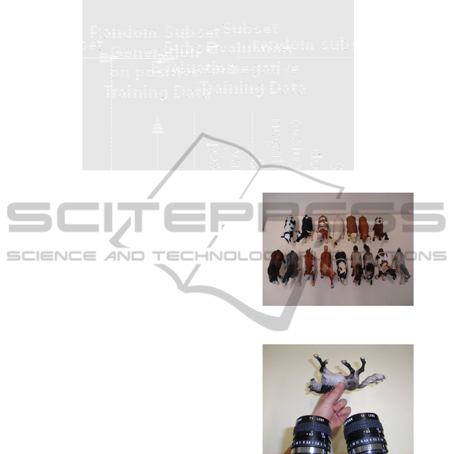
Figure 5: Random feature selection algorithm with validation.
experiments and results that show the possibility of
learning one 3D model per category.
5.1 Cross Validation
We use k-fold cross validation to evaluate our exper-
iments. Given a dataset D, this dataset is split into k
subsets of approximately equal size. In our case D =
{D
p
1
,...,D
p
S
1
,D
n
1
,...,D
n
S
2
} of positive and negative 3D
models and k = S
1
+ S
2
subsets. Consequently, one
subset is one 3D model. We train the classifier S
1
∗ S
2
times. In each iteration t ∈ 1,...,S
1
∗ S
2
, we leave out
one positive and one negative 3D model. So we train
on D\{D
p
i
,D
n
j
} ∀i = 1,...,S
1
and ∀ j = 1,...,S
2
and
test on D
p
i
and D
n
j
. In the cross validation we then
build the average over the results for the positive and
the negative test data.
5.2 Dataset
For our experiments we use our video databases con-
taining stereo image sequences of small toy objects of
the categories ‘horse’ and ‘cow’ (see Figure 6). The
videos are taken by a calibrated stereo rig. The ob-
jects are either manipulated naturally by hand in front
of a stereo camera system (see Figure 7) or they are
rotated using a turntable. The objects are manipu-
lated such that they are seen from all sides, show-
ing all aspects. 3D contour fragments are generated
using a multiview-stereo reconstruction scheme (see
Appendix A).
Figure 8 shows one example stereo frame pair
from a horse image sequence. Figure 2 shows an ex-
ample of a ‘3D contour cloud’ reconstruction of this
horse as described in Appendix A. Figure 9(a) is the
representation of the Gaussian Mixture Models of this
‘3D contour cloud’, Figure 9(c) shows selected par-
titions. Our dataset consists of nine horse ‘3D con-
Figure 6: Database of objects containing nine horses and
seven cows.
Figure 7: Stereo rig to capture the database. We use two
µEye 1220C cameras and Cosmicar/Pentax lenses with a
focal length of 12.5 mm. The baseline is approximately 6cm
(human eye distance), the vergence angle 5.5
o
. The frame
rate is 15 Hz. The size of the images is 480x752 px. For the
calibration of the stereo rig we use the Camera Calibration
Toolbox for Matlab (Bouguet).
tour clouds’ and seven cow ‘3D contour clouds’. This
leads to 9 ∗ 7 = 63 ‘leave-one-out’ experiments.
5.3 Experiments and Results
On the one hand, we show that the random feature se-
lection algorithm applied to positive training data can
be used to reduce outliers in 3D models. On the other
3D OBJECT CATEGORIZATION WITH PROBABILISTIC CONTOUR MODELS - Gaussian Mixture Models for 3D
Shape Representation
265
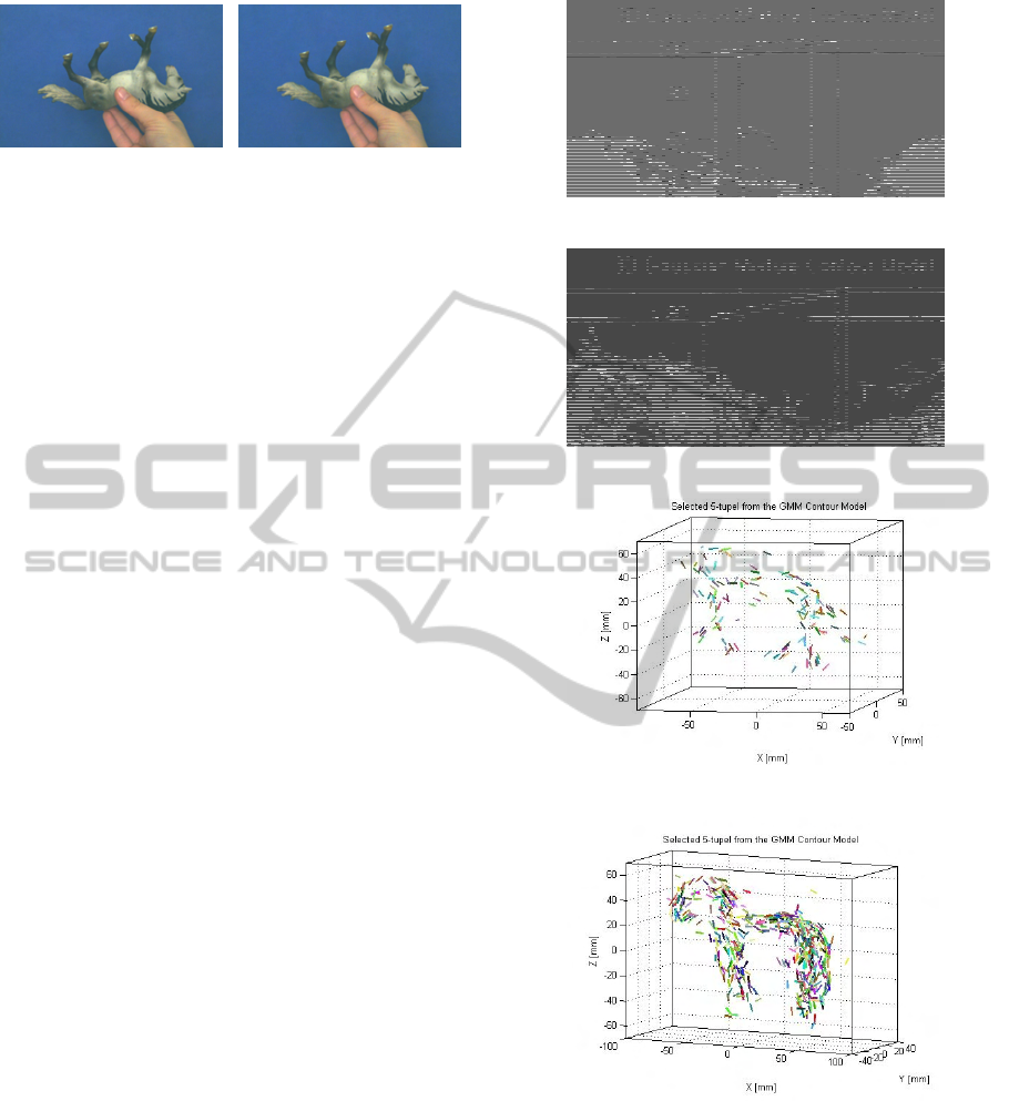
Figure 8: One example stereo frame pair of a horse. The
hand is masked using the method by (Unger et al., 2009).
hand, - and this is the main part of this section - we
show several experiments and results to achieve a 3D
model for the category ‘horse’ against the category
‘cow’.
5.3.1 Outlier Reduction
We mentioned in Section 3 that outliers in form of
wrongly reconstructed contour points always play an
important role in 3D reconstruction.
Noise is represented in the probability density
function as mentioned in Section 4. But there ex-
ist also outliers that result from the reconstruction
process and where a probability density function no
longer belongs to the shape of the object. By run-
ning the random feature selection only on the pos-
itive training data, we can see, that noisy parts can
be reduced significantly. Given nine horses, we ran-
domly select 1000 partitions of five mixture compo-
nents, where in each round the horse is randomly se-
lected out of a set of eight horses. Figure 9(a) and
Figure 9(b) show the Gaussian Mixture Models of two
horses. For visualization, the probability densities are
drawn by 3D lines given by their mean and the princi-
pal eigenvector. We can see that outliers exist, which
results from the ‘3D contour cloud’ generation. In
Figure 9(c) and Figure 9(d), we can see selected par-
titions of size 5 from the two horses which were dis-
criminant for all other horses. We can see, that most
of the discriminative probability densities are located
on the head, the back, and the tail of the horses. Fewer
densities are located on the legs, because of different
arrangements of the legs in the 3D horse models. Out-
liers have been significantly reduced.
5.3.2 Categorization
The aim of the following experiments is to learn a cat-
egory model ‘horse’ against ‘cows’. The challenge in
this learning experiments is the small inter-class dif-
ference between horses and cows. Our object catego-
rization system is validated using the cross-validation
scheme described in Section 5.1. We did several ex-
periments with different kinds of constraints (see Sec-
tion 4.2) on the random selection of partitions. We can
summarize the experiments as follows:
(a)
(b)
(c)
(d)
Figure 9: (a) & (c) GMM of a ‘3D contour cloud’ of a horse
and 28 partitions which have been selected. (b) & (d) GMM
of a ‘3D contour cloud’ of a horse and 128 partitions which
have been selected. We see, that the number of outliers is
significantly reduced. A partition of size 5 is represented by
the same color.
• Experiment 1: We randomly select partitions of
probability density functions from the 3D Gaus-
sian Mixture Contour Models of randomly se-
VISAPP 2011 - International Conference on Computer Vision Theory and Applications
266

lected horses of size 3 or 5, where we use the uni-
formity constraint (see Section 4.2). We perform
a cross validation experiment where the results of
this experiment are summarized in Table 1.
• Experiment 2: We randomly select partitions of
probability densities from the 3D Gaussian Mix-
ture Contour Models of randomly selected horses
of size 5 or 7, where we use no constraint. The
results of this experiment are summarized in Ta-
ble 2.
• Experiment 3: We randomly select partitions of
probability density functions from the 3D Gaus-
sian Mixture Contour Models of randomly se-
lected horses of size 5, where we use the local-
ity constraint. The results of this experiment are
summarized in Table 3.
For these experiments we typically choose γ
2
= 0.98
and l = 0. For Experiment 1 and Experiment 2 γ
1
=
0.2, for Experiment 3 γ
1
= 0.1. Too small γ
1
and
γ
2
do not handle intra-class variability, too large γ
1
and γ
2
do not handle inter-class difference. The result
tables (Table 1, Table 2, Table 3) contain seven en-
tries for each experiment. The average result of the
cross-validation for the positive training set ‘horse’
and the negative training set ‘cow’ is shown in the
first (µ
horse
) and the third (µ
cow
) row. Assuming a
normal distribution we can also compute the standard
deviations σ
horse
and σ
cow
, as well as a classification
threshold c thresh on whose basis we can decide if
a 3D test model is a ‘horse’ or a ‘cow’. c error
horse
and c error
cow
are the classification errors. Figure 10
shows a graphical representation of the results of Ex-
periment 1 - Partition (size 3). We can see that the two
categories are well separable. As the results show,
Experiment 1 and Experiment 2 perform better than
Experiment 3 with the local features. In Experiment 1
and Experiment 2, the classification errors are ≤ 21%.
The locality constraint seems to be less useful than a
uniform distribution. This result is not very surpris-
ing. Local features often have similar shape which
is not category specific, e.g. legs of horses and cows.
Only combinations with other local features (e.g. leg
and head of an animal) could give more discrimi-
nance. Moreover, we saw, that we have to learn longer
for Experiment 3 for the same number of partitions
than for Experiment 1 or Experiment 2. This is also
true for learning smaller partitions e.g. Experiment 1
- partition (size 3).
Figure 11 shows an example of a learned 3D cat-
egory model ‘horse’ from one training step of Exper-
iment 1 - partition (size 5). For this model we ran-
domly choose 1000 partitions, where 135 are found
to be discriminative for horses and not for cows. The
category model in Figure 11 has 135 partitions from
Table 1: Experiment 1: partition selection based on the uni-
formity constraint .
Partition (size 3) Partition (size 5)
µ
horse
0.7380 0.6781
σ
horse
0.1965 0.2328
µ
cow
0.3141 0.2481
σ
cow
0.2432 0.2191
c thresh 0.5248 0.4632
c error
horse
0.1401 0.1788
c error
cow
0.1922 0.1635
Table 2: Experiment 2: partition selection based on no con-
straint .
Partition (size 5) Partition (size 7)
µ
horse
0.7066 0.6648
σ
horse
0.2225 0.2271
µ
cow
0.2836 0.2325
σ
cow
0.2555 0.2302
c thresh 0.4912 0.4485
c error
horse
0.1660 0.1711
c error
cow
0.2090 0.1736
eight horses. All partitions are drawn in one model
without special aligning. We can see that discrimi-
nant probability density functions are located mainly
on the head, the back and the tail, fewer are on the
legs which is due to different arrangements of legs on
different training models. We can see a similar behav-
ior for Experiment 2. Figure 12 shows a learned 3D
category model ‘horse’ for Experiment 2 - partition
(size 7). The distribution of the probability density
functions is similar to that of Experiment 1, on head,
back, and tail. However, most of the densities are lo-
cated on the head of the horse.
6 CONCLUSIONS
AND OUTLOOK
We have presented a new approach for learning a 3D
Gaussian Contour Category Model using a probabilis-
tic framework based on Gaussian Mixture Models.
Instead of modeling the whole shape by a GMM and
computing a divergence between shapes, we represent
3D contour fragments by GMMs and apply a parti-
tioning on them. We show that it is possible to build
one single, pose-invariant 3D model per category in-
stead of building one model per significant view as
it is the case in 2D shape based models. Our results
demonstrate that we can learn one category against
another one, even when the inter-class difference is
small. The experiments show that global partitions
3D OBJECT CATEGORIZATION WITH PROBABILISTIC CONTOUR MODELS - Gaussian Mixture Models for 3D
Shape Representation
267
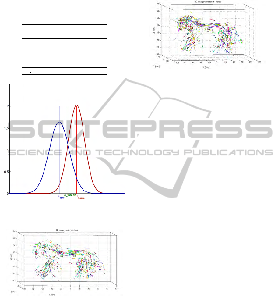
Table 3: Experiment 3: partition selection based on the lo-
cality constraint .
Partition (size 5)
µ
horse
0.5723
σ
horse
0.3304
µ
cow
0.2619
σ
cow
0.2907
c thresh 0.4462
c error
horse
0.3520
c error
cow
0.2643
Figure 10: Graphical representation of the results of Ex-
periment 1: Partition (size 3). The two categories are well
separable.
Figure 11: 3D category ‘horse’ model with 154 partitions
from eight horses of size 5 of Experiment 1. The probability
densities are drawn by 3D lines given by their mean and the
principal eigenvector.
(with a classification error ≤ 21%) are better suitable
for a category model than local features.
In our future work we plan to extend this ap-
proach to more object classes and to concentrate more
on modeling shape properties, e.g. relations between
transformations of probability density function and
pairwise relations. Here, also a hierarchical approach
Figure 12: 3D category ‘horse’ model with 142 partitions
from eight horses of size 7 of Experiment 2. The probability
densities are drawn by 3D lines given by their means and
their principal eigenvectors.
would make sense for building partitions. More-
over, we will improve learning by using a learning
algorithm after the random subset selection. A fur-
ther objective is to see if such a probabilistic 3D
model can be used for pose estimation in 2D images
(e.g. (Liebelt and Schmid, 2010)) or even for catego-
rization in 2D images. This would overcome known
problems of standard 2D categorization like sensitiv-
ity to pose/view changes.
ACKNOWLEDGEMENTS
This work was supported by the Austrian Science
Fund (FWF) under the doctoral program Confluence
of Vision and Graphics W1209.
REFERENCES
Belongie, S., Malik, J., and Puzicha, J. (2002). Shape
matching and object recognition using shape contexts.
IEEE Trans. PAMI, 24(4):509–522.
Bouguet, J.-Y. Camera calibration toolbox for matlab.
Cootes, T. (1999). A mixture model for representing shape
variation. Image and Vision Computing, 17(8):567–
573.
DeCarlo, D., Finkelstein, A., Rusinkiewicz, S., and San-
tella, A. (2003). Suggestive contours for conveying
shape. ACM Transactions on Graphics (Proc. SIG-
GRAPH), 22(3):848–855.
DeCarlo, D. and Rusinkiewicz, S. (2007). Highlight lines
for conveying shape. In International Symposium on
NPAR.
Ebrahimnezhad, H. and Ghassemian, H. (2007). Robust
motion and 3d structure from space curves. ISSPA
2007, pages 1–4.
Fabbri, R. and Kimia, B. B. (2010). 3D curve sketch: Flexi-
ble curve-based stereo reconstruction and calibration.
In Proceedings of the IEEE CVPR 2010.
VISAPP 2011 - International Conference on Computer Vision Theory and Applications
268

Gal, R., Shamir, A., and Cohen-Or, D. (2007a). Pose-
oblivious shape signature. IEEE TVCG, 13(2):261–
271.
Gal, R., Shamir, A., and Cohen-Or, D. (2007b). Pose-
oblivious shape signature. IEEE TVCG, 13(2):261–
271.
Goldberger, J., Gordon, S., and Greenspan, H. (2003). An
efficient image similarity measure based on approxi-
mations of KL-divergence between two gaussian mix-
tures. In Proc. on ICCV 2003, pages 487 –493 vol.1.
Iyer, N., Jayanti, S., Lou, K., Kalyanaraman, Y., and Ra-
mani, K. (2005). Three-dimensional shape searching:
state-of-the-art review and future trends. Computer-
Aided Design, 37(5):509–530.
Jian, B. and Vemuri, B. (2005). A robust algorithm for point
set registration using mixture of Gaussians. In Proc.
on ICCV 2005, volume 2, pages 1246 – 1251 Vol. 2.
Kazhdan, M., Funkhouser, T., and Rusinkiewicz, S. (2004).
Symmetry descriptors and 3D shape matching. In
Symposium on Geometry Processing.
Leibe, B., Leonardis, A., and Schiele, B. (2004). Combined
object categorization and segmentation with an im-
plicit shape model. In Workshop on Statistical Learn-
ing in Computer Vision, ECCV.
Leordeanu, M., Hebert, M., and Sukthankar, R. (2007).
Beyond local appearance: Category recognition from
pairwise interactions of simple features. In Proc. of
CVPR.
Liebelt, J. and Schmid, C. (2010). Multi-View Object Class
Detection with a 3D Geometric Model. In IEEE Con-
ference on CVPR.
Lowe, D. G. and Binford, T. O. (1983). Perceptual Orga-
nization as a Basis for Visual Recognition. In AAAI,
pages 255–260.
Mahmoudi, M. and Sapiro, G. (2009). Three-dimensional
point cloud recognition via distributions of geometric
distances. Graph. Models, 71(1):22–31.
Ohbuchi, R., Minamitani, T., and Takei, T. (2005). Shape-
similarity search of 3d models by using enhanced
shape functions. In IJCAT, volume 2005, pages 70–
85.
Ohtake, Y., Belyaev, A., and Seidel, H.-P. (2004). Ridge-
valley lines on meshes via implicit surface fitting.
ACM Trans. Graph., 23(3):609–612.
Opelt, A., Pinz, A., and Zisserman, A. (2006). A boundary-
fragment-model for object detection. In Proc. of
ECCV.
Osada, R., Funkhouser, T., Chazelle, B., and Dobkin, D.
(2002). Shape distributions. ACM Trans. Graph.,
21(4):807–832.
Park, J. S. and Han, J. H. (2002). Euclidean reconstruction
from contour matches. PR, 35:2109–2124.
Pauly, M., Keiser, R., and Gross, M. H. (2003). Multi-scale
feature extraction on point-sampled surfaces. Comput.
Graph. Forum, 22(3):281–290.
Peter, A. M. and Rangarajan, A. (2009). Information
Geometry for Landmark Shape Analysis: Unifying
Shape Representation and Deformation. Pattern Anal-
ysis and Machine Intelligence, IEEE Transactions on,
31(2):337–350.
Ross, S. M. (2005). Introductory Statistics. Academic
Press, Inc., Orlando, FL, USA.
Schweighofer, G., Segvic, S., and Pinz, A. (2008). On-
line/realtime structure and motion for general camera
models. IEEE WACV, pages 1–6.
Shilane, P., Min, P., Kazhdan, M., and Funkhouser, T.
(2004). The princeton shape benchmark. In Shape
Modeling International.
Shotton, J., Blake, A., and Cipolla, R. (2008). Multi-
Scale Categorical Object Recognition Using Contour
Fragments. IEEE Transactions on PAMI, 30(7):1270–
1281.
Sundar, H., Silver, D., Gagvani, N., and Dickinson, S.
(2003). Skeleton based shape matching and retrieval.
SMI ’03: Proceedings of the Shape Modeling Interna-
tional 2003, page 130.
Tangelder, J. and Veltkamp, R. (2007). A survey of content
based 3d shape retrieval methods. Multimedia Tools
and Applications.
Unger, M., Mauthner, T., Pock, T., and Bischof, H. (2009).
Tracking as segmentation of spatial-temporal volumes
by anisotropic weighted tv. In 7th International Con-
ference, EMMCVPR, volume 5681 of LNCS, Bonn,
Germany. Springer.
Wang, F., Vemuri, B. C., Rangarajan, A., and Eisenschenk,
S. J. (2008). Simultaneous Nonrigid Registration of
Multiple Point Sets and Atlas Construction. IEEE
Trans. PAMI, 30(11):2011–2022.
Xu, L. and Jordan, M. I. (1996). On convergence properties
of the em algorithm for gaussian mixtures. Neural
Comput., 8(1):129–151.
APPENDIX A
In this Appendix, we briefly describe how we build
3D contour fragments from stereo image sequences -
so called ‘3D contour clouds’. However, we point out,
that the method described in Section 4 will work on
all kinds of contours independent of the reconstruc-
tion method, as long as the 3D contour fragments rep-
resent the shape of a category.
In our approach, we combine stereo correspon-
dence on contour fragments and a robust Structure
and Motion analysis. The ‘3D contour cloud’ stereo
reconstruction process consists of several steps:
1. Image Acquisition - Dataset Generation. We
capture several stereo videos of different hand-
held objects which are manipulated in front of a
stereo rig (see an example in Section 5.2).
2. Preprocessing. To reconstruct just contours of
the hand-held objects and not contours of the
3D OBJECT CATEGORIZATION WITH PROBABILISTIC CONTOUR MODELS - Gaussian Mixture Models for 3D
Shape Representation
269

hand, we first have to mask the hand in the stereo
videos of hand-held objects. Here, we use a seg-
mentation algorithm based on variational methods
(Unger et al., 2009), which gives us a precise hand
segmentation. Features that belong to the hand are
subsequently ignored.
3. Contour Fragment Extraction. We apply the
Canny edge detection algorithm (subpixel accu-
racy) to extract contour fragments in the left and
the right frame of a stereo frame pair. Then, a
linking algorithm based on smoothing constraints
(Leordeanu et al., 2007) is used to obtain long,
connected 2D contour fragments.
4. Stereo Correspondence. For the reconstruction
of 3D contour fragments we need to find corre-
sponding 2D contour fragments and point corre-
spondences on them. We identify stereo corre-
spondences in two steps. First, we match contour
fragments in the right and the left stereo frame
pair. Next, we compute point correspondences on
these matches. In this step we combine 2D Shape
Context (Belongie et al., 2002) and epipolar in-
formation, which is available by the stereo cali-
bration.
5. Stereo Reconstruction. Based on the contour
point correspondences we reconstruct the 3D con-
tour fragments using the ‘Object Space Error for
General Camera Models’ (Schweighofer et al.,
2008).
6. S+M Analysis. The robust S+M analysis uses
point features and is based on the work by
(Schweighofer et al., 2008).
VISAPP 2011 - International Conference on Computer Vision Theory and Applications
270
