
EFFICIENT MOTION DEBLURRING FOR INFORMATION
RECOGNITION ON MOBILE DEVICES
Florian Brusius, Ulrich Schwanecke and Peter Barth
Hochschule RheinMain, Unter den Eichen 5, 65195 Wiesbaden, Germany
Keywords:
Image processing, Blind deconvolution, Image restoration, Deblurring, Motion blur estimation, Barcodes,
Mobile devices, Radon transform.
Abstract:
In this paper, a new method for the identification and removal of image artifacts caused by linear motion
blur is presented. By transforming the image into the frequency domain and computing its logarithmic power
spectrum, the algorithm identifies the parameters describing the camera motion that caused the blur. The
spectrum is analysed using an adjusted version of the Radon transform and a straightforward method for
detecting local minima. Out of the computed parameters, a blur kernel is formed, which is used to deconvolute
the image. As a result, the algorithm is able to make previously unrecognisable features clearly legible again.
The method is designed to work in resource-constrained environments, such as on mobile devices, where it
can serve as a preprocessing stage for information recognition software that uses the camera as an additional
input device.
1 INTRODUCTION
Mobile devices have become a personal companion
in many people’s daily lives. Often, mobile applica-
tions rely on the knowledge of a specific context, such
as location or task, which is cumbersome to provide
via conventional input methods. Increasingly, cam-
eras are used as alternative input devices providing
context information – most often in the form of bar-
codes. A single picture can carry a large amount of
information while at the same time, capturing it with
the integrated camera of a smartphone is quick and
easy. The processing power of smartphones has sig-
nificantly increased over the last years, thus allowing
mobile devices to recognise all kinds of visually per-
ceptible information, like machine-readable barcode
tags and theoretically even printed text, shapes, and
faces. This makes the camera act as an one-click
link between the real world and the digital world in-
side the device (Liu et al., 2008). However, to reap
the benefits of this method the image has to be cor-
rectly recognised under various circumstances. This
depends on the quality of the captured image and is
therefore highly susceptible to all kinds of distortions
and noise. The photographic image might be over- or
underexposed, out of focus, perspectively distorted,
noisy or blurred by relative motion between the cam-
era and the imaged object. Unfortunately, all of those
problems tend to occur even more on very small cam-
eras. First, cameras on smartphones have very small
image sensors and lenses that are bound to produce
lower quality images. Second, and more important,
the typical single-handed usage and the light weight
of the devices make motion blur a common problem
of pictures taken with a smartphone. In many cases,
the small tremor caused by the user pushing the trig-
ger is already enough to blur the image beyond ma-
chine or human recognition.
Blurry image taken by user Preprocessing (blur removal)
4915355604303
Information recognition
Figure 1: Use of the image deblurring algorithm as a pre-
processing stage for information recognition software.
In order to make the information that is buried in
blurry images available, the artefacts caused by the
blur have to be removed before the attempt to extract
the information. Such a preprocessing method should
run in an acceptable time span directly on the de-
vice. In this paper, we present a method that identifies
and subsequently removes linear, homogeneous mo-
tion blur and thus may serve as a preprocessing stage
for information recognition systems (see figure 1).
7
Brusius F., Schwanecke U. and Barth P..
EFFICIENT MOTION DEBLURRING FOR INFORMATION RECOGNITION ON MOBILE DEVICES.
DOI: 10.5220/0003321200070018
In Proceedings of the International Conference on Imaging Theory and Applications and International Conference on Information Visualization Theory
and Applications (IMAGAPP-2011), pages 7-18
ISBN: 978-989-8425-46-1
Copyright
c
2011 SCITEPRESS (Science and Technology Publications, Lda.)

2 RELATED WORK
In the last thirty-five years, many attempts have been
made to identify and remove artefacts caused by im-
age blur. Undoing the effects of linear motion blur
involves three basic steps that can be considered as
more or less separate from each other: Calculating
the blur direction, calculating the blur extent, and fi-
nally using these two parameters to deconvolute the
image. Since the quality of the deconvolution is
highly dependent on the exact knowledge of the blur
kernel, most publications focus on presenting new
ways for blur parameter estimation. While some of
the algorithms are developed to work upon a series
of different images taken of the same scene (Chen
et al., 2007; Sorel and Flusser, 2005; Harikumar and
Bresler, 1999), the method in this paper attempts to
do the same with a single image.
2.1 Blur Angle Calculation
Existing research can be divided into two groups: One
that strives to estimate the blur parameters in the spa-
tial image domain and another that tries to do the
same in the frequency domain.
The former is based on the concept of motion
causing uniform smear tracks of the imaged objects.
(Yitzhaky and Kopeika, 1996) show that this smear-
ing is equivalent to the reduction of high-frequency
components along the direction of motion, while it
preserves the high frequencies in other directions.
Thus, one can estimate the blur angle by differen-
tiating the image in all directions and determining
the direction where the total intensity of the image
derivative is lowest. However, this approach works
best when the imaged objects are distinct from the
background, so that the smears will look like distinct
tracks. It also assumes that the original image has
similar local characteristics in all directions. Such
methods suffer from relatively large estimation errors
(Wang et al., 2009). They also need a lot of computa-
tion time and therefore are not applicable to real time
systems.
A more common approach is the blur direction
45°
Figure 2: Image of a barcode blurred by linear camera mo-
tion in an angle of 45° and the resulting features in its loga-
rithmic power spectrum.
identification in the frequency domain. (Cannon,
1976) showed that an image blurred by uniform lin-
ear camera motion features periodic stripes in the fre-
quency domain. These stripes are perpendicular to
the direction of motion (see figure 2). Thus, know-
ing the orientation of the stripes means knowing the
orientation of the blur. In (Krahmer et al., 2006), an
elaborate overview of the diverse methods for esti-
mating linear motion blur in the frequency domain is
presented. One possibility to detect the motion an-
gle is the use of steerable filters, which are applied to
the logarithmic power spectrum of the blurred image.
These filters can be given an arbitrary orientation and
therefore they can be used to detect edges of a cer-
tain direction. Since the ripples in the image’s power
spectrum are perpendicular to the direction of motion
blur, the motion angle can be obtained by seeking the
angle with the highest filter response value (Rekleitis,
1995). Unfortunately, this method delivers very in-
accurate results. Another method of computing the
motion direction analyses the cepstrum of the blurred
image (Savakis and Easton Jr., 1994; Chu et al., 2007;
Wu et al., 2007). This is based on the observation that
the cepstrum of the motion blur point spread function
(PSF) has large negative spikes at a certain distance
from the origin, which are preserved in the cepstrum
of the blurred image. In theory, this knowledge can
be used to obtain an approximation of the motion an-
gle by drawing a straight line from the origin to the
first negative peak and computing the inverse tangent
of its slope. However, this method has two major
disadvantages. First, it only delivers good results in
the absence of noise, because image noise will sup-
press the negative spikes caused by the blur. And sec-
ond, calculating the cepstrum requires an additional
inverse Fourier transform, which is computationally
expensive. A third approach is the use of feature
extraction techniques, such as the Hough or Radon
transform. These operations detect line-shaped struc-
tures and allow for the determination of their orien-
tations (Toft, 1996). The Hough transform, as it is
used in (Lokhande et al., 2006), requires a prelimi-
nary binarisation of the log spectrum. Since the high-
est intensities concentrate around the center of the
spectrum and decrease towards its borders, the bina-
risation threshold has to be calculated separately for
each pixel, which can become computationally pro-
hibitive. Another issue is that the stripes tend to melt
into each other at the origin and thus become indis-
tinct, which makes finding an adaptive thresholding
algorithm that is appropriate for every possible ripple
form a difficult, if not impossible task (Wang et al.,
2009). The Radon transform is able to perform di-
rectly upon the unbinarised spectrum and is therefore
IMAGAPP 2011 - International Conference on Imaging Theory and Applications
8

much more practical for time-critical applications. As
a result, it delivers a two-dimensional array in which
the coordinate of the maximum value provides an esti-
mate of the blur angle. According to (Krahmer et al.,
2006), the Radon transform delivers the most stable
results. However, this method needs a huge amount
of storage space and computation time.
2.2 Blur Length Calculation
The estimation of the blur extent in the spatial image
domain is based on the observation that the derivative
of a blurred image along the smear track emphasises
the edges of the track which makes it possible to iden-
tify its length (Yitzhaky and Kopeika, 1996). Again,
this method highly depends on distinctively visible
smear tracks and is therefore very unstable. Most
of the algorithms estimate the blur length in the fre-
quency domain, where it corresponds to the breadth
and frequency of the ripples. The breadth of the cen-
tral stripe and the gaps between the ripples are in-
versely proportional to the blur length. To analyse
the ripple pattern, usually the cepstrum is calculated.
One way of computing the blur extent is to estimate
the distance from the origin where the two negative
peaks become visible in the cepstrum. After rotat-
ing the cepstrum by the blur angle, these peaks ap-
pear at opposite positions from the origin and their
distance to the y-axis can easily be determined (Chu
et al., 2007; Wu et al., 2007). Another way collapses
the logarithmic power spectrum onto a line that passes
through the origin at the estimated blur angle. This
yields a one-dimensional version of the spectrum in
which the pattern of the ripples becomes clearly vis-
ible, provided that the blur direction has been calcu-
lated exactly enough. By taking the inverse Fourier
transform of this 1-D spectrum, which can be called
the 1-D cepstrum, and therein seeking the coordinate
of the first negative peak, the blur length can be esti-
mated (Lokhande et al., 2006; Rekleitis, 1995). As
with the angle estimation, these two methods have
their specific disadvantages: In the first method, cal-
culating the two-dimensional cepstrum is a compara-
tively expensive operation, while the second method
is once again highly susceptible to noise.
2.3 Image Deblurring
Knowing the blur parameters, an appropriate PSF can
be calculated. This blur kernel then can be used to re-
construct an approximation of the original scene out
of the distorted image (Krahmer et al., 2006). Un-
fortunately, traditional methods like Wiener or Lucy-
Richardson filter tend to produce additional artefacts
of their own in the deconvoluted images (Chalkov
et al., 2008). These artefacts particularly occur at
strong edges and along the borders of the image.
Some methods have been developed to overcome that
issue, such as in (Shan et al., 2008), where a new
model for image noise is presented. However, these
methods always involve some sort of iterative optimi-
sation process, which is repeated until the result con-
verges towards an ideal. This makes them inappropri-
ate for the use in time-critical applications. Luckily,
there is no need to get rid of all the artefacts, as long
as the information contained in the image is recognis-
able. However, it has to be taken into account that the
deconvolution artefacts may still hinder or complicate
the recognition process.
3 THE IMAGE DEGRADATION
MODEL
In order to support the elimination or reduction of
motion blur, a mathematical model that describes this
degradation is needed. When a camera moves over a
certain distance during exposure time, every point of
the pictured scene is mapped onto several pixels of the
resulting image and produces a photography that is
blurred along the direction of motion. This procedure
can be regarded as some sort of distortion of the un-
blurred original image, i.e. the picture taken without
any relative movement between the camera and the
imaged scene. The distortion can be modelled as a lin-
ear filter function h(u,v) that describes how a point-
shaped light source would be mapped by the photog-
raphy and which is therefore called the point spread
function (PSF). Thus, the blurring of an original im-
age f (u,v) (see figure 3) equates to the linear convo-
lution ∗ with the adequate PSF (Cannon, 1976). In
the case of linear homogeneous motion blur, this PSF
is a one-dimensional rectangular function (Lokhande
et al., 2006). The PSF looks like a line through the
point of origin with the angle ϕ to the x-axis, equal
to the direction of motion, and the length L, equal to
the distance one pixel travels along this direction of
motion. The coefficients in h(u,v) sum up to 1, thus
the intensity being
1
/L along the line and 0 elsewhere.
With the knowledge of the correct motion parameters,
the PSF can be calculated via
h(u,v) = (1)
=
1
L
if (u,v)
sinϕ
cosϕ
!
= 0 and u
2
+ v
2
<
L
2
2
0 otherwise .
EFFICIENT MOTION DEBLURRING FOR INFORMATION RECOGNITION ON MOBILE DEVICES
9

It has to be taken into account that in the majority
of cases, the undistorted original image is deranged by
additional, signal-independent noise. This noise can
be modelled as an unknown random function n(u,v),
which is added to the image. Hence, the blurred im-
age i(u,v) can be described as
i(u,v) = f (u,v)∗h(u,v) + n(u,v) . (2)
Because the convolution becomes a multiplication in
the frequency domain, the Fourier transform of the
blurred image equates to
I(m, n) = F(m,n) ·H(m,n) + N(m,n) . (3)
This multiplication could theoretically be reversed
by pixel-wise division, so with the knowledge of
the proper PSF, the undistorted original image could
be obtained through the inverse Fourier transform.
This procedure is often referred to as inverse filter-
ing (Gonzalez and Woods, 2008). However, this only
works properly under the assumption that there is zero
noise. In the presence of noise, only an approximation
ˆ
F of the transformed original image can be obtained,
which equals to
ˆ
F =
I(m, n)
H(m,n)
=
F(m,n) ·H(m,n) + N(m,n)
H(m,n)
= F(m,n) +
N(m,n)
H(m,n)
.
(4)
This shows that
ˆ
F cannot be reconstructed without
the knowledge of the transformed noise function N.
In addition, the small coefficients in H(m,n) make
the term
N(m,n)
/H(m,n) very large and superpose the ac-
tual original image beyond recognition (Gonzalez and
Woods, 2008). To avoid that, a method of inverse fil-
tering is needed that explicitly takes the noise signal
into consideration. The Wiener deconvolution is such
a method, which is based on the well known Wiener
filter (Wiener, 1949) for noise suppression in signal
processing.
*
=
Figure 3: Motion blur can be modelled as a linear convolu-
tion with an appropriate PSF.
4 THE IMAGE DEBLURRING
ALGORITHM
In the algorithm presented in this paper, a given
blurred input image is analysed to determine the
direction and length of the camera movement that
caused the blur. These two motion parameters are
used to calculate a point spread function modelling
the blur. Regarding the blur as a linear convolution
of the original image with that blur kernel, it can be
removed by reversing this operation. The algorithm
focuses on efficient computation and is therefore suit-
able for resource-limited environments.
First, in section 4.1 a preprocessing step, which
converts a relevant part of the respective greyscale
image to the frequency domain with FFT, is intro-
duced. Then, in section 4.2 the blur direction is deter-
mined by performing a Radon transform on the log-
arithmic power spectrum of the blurred image. The
power spectrum features some ripples in its centre,
which run perpendicular to the direction of motion.
The computation time of the Radon transform is sig-
nificantly decreased by customising it to fit the struc-
tural conditions of the spectrum. Next, in section 4.3
the blur length is estimated by measuring the breadth
of the central ripple within the log spectrum, which is
inversely proportional to the sought-after blur length.
This is done by collapsing the spectrum onto a line
that passes through its origin at an estimated blur an-
gle. Then the resulting one-dimensional log spec-
trum is analysed to find the first significant local min-
imum. This approach does not require any further
costly Fourier transforms. In the last step in sec-
tion 4.4, the PSF is calculated and a simple Wiener
filter is used to deconvolute the image.
Figure 4 shows an overview of the algorithm. It
also denotes the additional costly segmentation of the
image that is required if instead of the Radon trans-
form the Hough transform is used to detect the blur
direction.
4.1 Preprocessing
Estimating the blur parameters requires some pre-
processing. First, the colour image obtained by
the smartphone camera is converted into an 8 bit-
greyscale picture. This can be done by averaging the
colour channels or by weighting the RGB-parts ac-
cording to the luminance perception of the human eye
(Burger and Burge, 2008).
i
0
(u,v) = 0.30 ·i
R
(u,v)+0.59 ·i
G
(u,v)+0.11 ·i
B
(u,v)
(5)
Next, a square section is cut out of the centre of the
image. For the FFT to be applicable, this size has to
IMAGAPP 2011 - International Conference on Imaging Theory and Applications
10

Preprocessing
Blurry input image
8 bit-grayscale image Square image area
Hough-Transformation
Radon-Transformation
Segmentierung
(White-Schwellwert)
Hough-Transformation
Radon-Transformation
Auswertung des Akkumulator-Arrays
Blur direction determination
Hough transform
Radon transform
Segmentation
(White thresholding)
Hough transform
Radon transform
Blur length
determination
1-D spectrum
Auswertung des Akkumulator-Arrays
Estimation of the
breadth of the central
peak
length L
Deconvolution
Auswertung des
Akkumulator-Arrays
Fourier transform of
original image and
point spread function
Calculation of the
point spread function
Wiener-filter
Inverse Fourier transform
Quadrant swap
Masking with Hanning
window
Fourier transform, quadrant swap & logarithmic power spectrum
Analysis of the accumulator array angle φ
Figure 4: Overview of the image deblurring algorithm.
be a power of two. In practise, sizes of 512 ×512
and 256 ×256 pixels have shown to maintain a rea-
sonable balance between stable high quality results
and computational cost. The period transitions from
one image border to the next often lead to high fre-
quencies, which become visible in the image’s power
spectrum as vertical and horizontal lines. Since these
lines may distract from or even superpose the stripes
caused by the blur, they have to be eliminated by ap-
plying a windowing function before transforming the
image. The Hanning window offers a good trade-off
between forming a smooth transition towards the im-
age borders and preserving a sufficient amount of im-
age information for the parameter estimation. For a
square image of size M, the Hanning window is cal-
culated as (Burger and Burge, 2008)
w
Hanning
(u,v) =
(
0.5 ·cos(πr
u,v
+ 1) if 0 ≤r
u,v
≤ 1
0 otherwise
with
r
u,v
=
s
2u
M
−1
2
+
2v
M
−1
2
.
(6)
After that step, the windowed image can be trans-
ferred into the frequency domain by performing a
FFT. To facilitate the identification of particular fea-
tures of the Fourier spectrum, its power spectrum is
computed. In its basic form, the power spectrum is
defined as the absolute value of the Fourier trans-
formed image. However, because the coefficients of
the Fourier spectrum decrease rapidly from its cen-
ter towards the borders, it can be difficult to identify
local differences. Taking the logarithm of the power
spectrum s(u,v) = log|I(m,n)| helps to balance this
rapid decrease. In order to obtain a centred version of
the spectrum, its quadrants have to be swapped di-
agonally. Since the interesting features are around
the centre of the spectrum, the following operations
can be performed upon a centred 256 ×256-window,
which reduces computation time.
4.2 Blur Direction Determination
As a result of the above operations, the power spec-
trum exhibits a pattern of stripes parallel to a line
passing through its origin at an angle θ, which cor-
responds to the motion angle ϕ as θ = −ϕ. Thus, es-
timating the direction of these stripes means knowing
the motion angle. To do so, a Radon transform is per-
formed. This is done by shooting a certain amount
of parallel rays for each possible angle θ through
the image, adding up the intensities of the pixels hit
by each ray and subsequently storing the sums in a
two-dimensional accumulator array. The high inten-
sity values along the sought-after stripes lead to local
maxima within this array, and the corresponding ar-
ray indices reveal the parameters (radius and angle)
of the detected lines. The precision of the algorithm
depends on how fine the angle domain θ = 0 . . .π is
divided into a number of n
θ
steps. 360 steps provide
an accuracy of 0.5°, which is sufficient for image re-
construction and subsequent information extraction.
In the general case where the position of the
sought-after feature is unknown, there is no alterna-
tive but to try every possible distance for each angle
(see figure 6(a)). Yet with the previous knowledge
that the central stripe runs through the origin, the ra-
dius is always 0 and the complexity of the procedure
can be significantly decreased. Theoretically, all what
has to be done is to shoot one ray per angle through
the origin of the spectrum and determine the angle
with the highest sum (see figure 6(b)).
Unfortunately, this method usually fails in prac-
tise. Periodic structures are common in e.g. barcodes
and high-contrast edges occur for example along the
border of a white sheet of paper photographed against
a dark background. In the spectrum they manifest as
EFFICIENT MOTION DEBLURRING FOR INFORMATION RECOGNITION ON MOBILE DEVICES
11

86°
94°
0° 22,5° 45° 67,5° 90° 112,5° 135° 157,5° 180°
Figure 5: The periodic structures of the barcode lead to ad-
ditional features in the power spectrum and create distract-
ing maxima in the Radon accumulator array.
additional lines (see figure 5). Since these distracting
parts tend to have very high frequencies, they can eas-
ily lead to wrong estimations. Therefore, a criterion is
needed which helps to separate the “wrong” features
from the “right” ones. Fortunately, the breadth of the
central stripe caused by the blur is inversely propor-
tional to the blur length. This means that for typical
cases of motion blur up to 50-70 pixels, the blur stripe
is much broader than the distracting other stripes. At
the same time, it is also more diffuse, meaning that
it spreads its energy over its breadth. The correct an-
gle can reliably be estimated by looking for maxima
within the expected breadth from the origin only (see
figure 6(c)). This is a nontrivial problem, because the
blur length and with it the expected breadth b are not
known. Since taking a value for b that is significantly
larger than the actual breadth would lead to an in-
accurate estimation, the best result can be achieved
by choosing b according to the largest expected blur
length (which corresponds to the smallest expected
ripple breadth). The blur length is equal to the size
of the spectrum divided by the half of b. Hence, for
a length of 60 pixels, b equates to
1
30
of the spectrum
width.
(a) (b) (c)
Figure 6: Three different versions of the Radon transform.
The arrows denote the rays shot through the image for one
particular angle. In (a), every single possible radius is
taken into account, whereas (b) and (c) are individually cus-
tomised to the expected structure of the power spectra.
The result is an array with n
θ
·b sums. Determin-
ing the correct blur angle out of this array is done by
searching for the w consecutive angles whose sums
add up to the highest total sum. Each of these sums
consists of b single values, according to the number
of rays sent through the image for each angle. Having
found these w angles, the maximum out of all w ·b
single values is determined. The angle to whose sum
this maximum value has contributed is the desired an-
gle of camera motion. A range of 3° has proven to
be sufficiently large to ensure that the correct angle is
selected, so that w can be calculated out of the angle
resolution n
θ
.
w =
n
θ
180
·3 (7)
4.3 Blur Length Determination
The blur length is also calculated by analysing the
logarithmic power spectrum of the blurred image.
Here, it is the breadth of the central ripple running
through the origin that has to be estimated. This
breadth is inversely proportional to the blur extent and
therefore can be used to calculate it. Unlike the ma-
jority of other algorithms, the estimation requires no
further Fourier transform. To determine the breadth
of the central stripe, a one-dimensional version of the
spectrum is calculated. This is done by collapsing
the intensity values of the spectrum onto a line run-
ning through the origin perpendicular to the blur rip-
ples. The intensity of each pixel is summed up in an
array according to its distance d from that line. In
order to do so, d has to be discretised first. Since
simple rounding may lead to imprecise results, (Rek-
leitis, 1995) proposes another approach where the in-
tensities are proportionately divided into two array in-
dexes according to the decimal places of their dis-
tances from the projection line. He also suggests to
normalise the projected spectrum by dividing each
sum by the amount of pixels that went into it. That
way, the sums do not necessarily decrease towards
the borders of the array, because fewer pixels con-
tribute to them. In addition to these two improve-
ments, (Krahmer et al., 2006) proposes to mirror the
array in its centre and to add the values to the respec-
tive other side. Due to the fact that the blur ripples
should be symmetric, this suppresses noise and at the
same time clarifies the interesting features.
The resulting 1-D spectrum exhibits a prominent
peak in its centre which matches the central blur rip-
ple in the 2-D spectrum (see figure 7). The zeros, or
rather the gaps, between the individual stripes man-
ifest as local minima in the collapsed spectrum. To
identify the maximum in the centre of the spectrum,
a search to the right (either direction would be possi-
ble because of the symmetry) is performed until the
values become higher instead of smaller.
P(x
0
) < P(x
0
+ 1) (8)
Out of this first local minimum x
0
, one easily can cal-
culate the breadth of the blur ripple by doubling its
IMAGAPP 2011 - International Conference on Imaging Theory and Applications
12

(a) (b)
Figure 7: The log power spectrum of a blurred image (a)
and the plot of its projected 1-D spectrum (b).
distance to the maximum. Unfortunately, this sim-
ple approach usually fails in the presence of noise.
With blur that has been developed under realistic con-
ditions, small deflections show up in the spectrum.
Thus, the collapsed spectrum is not monotonically de-
creasing up to the sought-after first local minimum
and the approach described in (8) is bound to fail. To
solve this problem, we propose to define a distance s
within which the values must not become bigger than
at the potential minimum.
P(x
0
) < P(x
0
+ 1) < P(x
0
+ s) (9)
Since the parallel ripples in the spectrum become
smaller and more dense to the same degree the caus-
ing movement is faster, the choice of a proper value
for s is not an easy one. On the one hand, it has to
be larger than the maximal breadth of the noise de-
flections it strives to suppress. On the other hand,
it has to be smaller than the minimal breadth of the
next ripple, which is half as broad as the one in the
centre. This means that s has to be individually com-
puted according to the characteristics of the present
spectrum. With increasingly larger blur lengths, the
values in the spectrum decline more rapidly towards
the sides. This is why the calculation of the slope m
between two points Q
1
= (x
1
,y
1
) and Q
2
= (x
2
,y
2
),
which both lie on the central peak, is a promising ap-
proach. To be on the safe side, we presume a maxi-
mal blur length of 100 pixels, which would make the
breadth of the entire peak
1
50
of the width
√
2M of the
spectrum. Hence, x
1
is set to be at the centre
M
/
√
2
and x
2
at a distance of
1
100
of the spectrum width from
there.
m =
y
2
−y
1
x
2
−x
1
=
P(x
2
) −P(x
1
)
1
100
√
2M
(10)
The resulting slope m grows with increasingly
larger blur lengths. At the same time, the deflections
become smaller as the slope becomes steeper, which
means that smaller blur lengths are more susceptible
to noise than larger ones. Thus, for determining s, we
use the reciprocal of m, multiplied by an appropriate
correction factor f :
s =
1
m
· f . (11)
For a spectrum with a size of 512 × 512 pixels, we
found that dividing the slope by a correction factor of
5 worked best. Since the breadths of the peaks depend
on the size M of the projected power spectrum, this
results in a correction factor of f =
M
2560
:
s =
1
m
· f =
1
m
·
M
512 ·5
=
M
2560 ·m
. (12)
When the correct minimum x
0
has been found accord-
ing to equation (9), the breadth b of the peak is calcu-
lated as
b = 2 ·
x
0
−
M
√
2
. (13)
Because b is inversely proportional to the length L of
the camera motion, the reciprocal of b is used. L is
then calculated by dividing the size of the spectrum
by the half of b.
L =
2M
b
(14)
It is possible that the algorithm fails to detect a local
minimum. This is mostly due to a faulty calculation
of the distance s or the collapsed spectrum exhibiting
no prominent peaks. The latter is the case when the
angle has not been estimated exactly enough in the
previous step, which leads to an incorrect projection
line orientation.
4.4 Deconvolution
Knowing the two blur parameters, an adequate PSF
can be calculated according to equation (1). Then
both the PSF and the original, unaltered image have
to be transformed into the frequency domain so that
the deconvolution can be carried out. The Wiener de-
convolution filter as it is presented in (Lokhande et al.,
2006) is given by
ˆ
F =
H
∗
(m,n) ·I(m,n)
H
∗
(m,n) ·H(m,n) + K
, (15)
where H
∗
(m,n) is the complex conjugate of H(m,n)
and K is a constant that can be approximated by the
reciprocal image width
1
/B. In order to obtain the
reconstructed, deblurred image, the result eventually
has to be transformed back into the image domain.
Provided that the information in the pictured ob-
ject consists solely of monochrome elements, it might
be reasonable to binarise the reconstructed image.
Good results can be achieved with the thresholding
EFFICIENT MOTION DEBLURRING FOR INFORMATION RECOGNITION ON MOBILE DEVICES
13

algorithms of White (White and Rohrer, 1983) and
Bernsen (Sezgin and Sankur, 2004). Since most of the
locally-adaptive thresholding methods require a lot of
computation time, this method is better used in envi-
ronments that are not time critical. However, if the
photo is consistently lit so that a viable global thresh-
old can be found, the method of Otsu (Otsu, 1979)
might also be applicable.
5 EVALUATION
In order to evaluate how accurate and reliable the mo-
tion parameter estimation works, two different classes
of input data have been used. The first category con-
sisted of images with artificially generated motion
blur. To do so, 11 different motifs had each been con-
voluted with 30 different PSFs. These PSFs had been
constructed from all possible combinations out of five
different, randomly chosen angles and six different,
likewise random lengths according to the definition
given by equation (1). This way, a total of 330 test
images were created. The original motifs comprised
real photography as well as completely digitally cre-
ated pictures, all of a size of 512 × 512 pixels.
Nine of the images showed different kinds of bar-
codes. The benefit of artificially created blur is that
the exact motion parameters are known beforehand
and can therefore easily be compared to the ones de-
termined by the algorithm. Yet it can not predict
whether the method works for photos taken under real
conditions. Hence, the second class consisted of real,
unaltered photographs. For these pictures, five differ-
ent barcodes had each been photographed five times.
In order to simulate realistic conditions, they were
made using a smartphone camera, manually moving
the phone in different speeds and angles during expo-
sure time. The shots were also taken under different
light conditions in order to vary the shutter speed.
5.1 Artificial Blur
For the artificially blurred images, the angle estima-
tion continuously produced stable results. The algo-
rithm could estimate the angles up to an accuracy of
5° for 92.71% of the test images. In most of the cases
where the estimation delivered incorrect results, this
was caused by additional features in the power spec-
trum induced by periodic structures or high-contrast
edges. The accuracy of the angle estimation is to
some degree dependent on the intensity of the blur:
If the ray within which the Radon transform sums up
the intensity values is smaller than the stripe it strives
to detect, multiple maxima occur at adjacent angles.
Since shorter blur lengths lead to broader stripes, the
accuracy decreases with the blur length, as can be
seen in table 1. Only taking into account pictures with
blur lengths greater than 50 pixels leads to an increase
of the detection rates for 0.5° accuracy of 40% of the
images. Out of the pictures with blur lengths greater
than 30 pixels, nearly 100% could be detected cor-
rectly with an accuracy of 4°.
The blur length estimation also worked reliably,
provided that the angle had been calculated correctly.
In the case of an exact angle estimation in the range
of 0.5° around the desired value, 95.73% of the blur
lengths could be determined with an accuracy up to
5 pixels. As shown in table 2, this rate decreases to
79.43% for an angle estimation accuracy of 5°. Given
these numbers, the percentage of images where both
the angle and the length could be estimated with an
accuracy of up to 5° or 5 pixels, is 73.56%. Never-
theless, the high portion of correctly estimated blur
lengths with the exact knowledge of the blur angle
shows that the method for blur length estimation pre-
sented in this paper works well. The accuracy how-
ever decreases for greater blur lengths, which is once
again due to the breadth of the central ripple: In a
spectrum of the size of 256 pixels, it is 26 pixels broad
for a blur length of 20 pixels. If the blur length is dou-
bled to 40 pixels, the breadth is halved accordingly to
13 pixels. For a blur length of 80 pixels, the stripe is
merely 6 pixels broad. The breadth of the ripple con-
verges towards the resolution limit and the accuracy
with which it can be determined inevitably decreases.
5.2 Real Blur
To allow the verification of the blur parameters es-
timated for photos taken under real conditions, the
angles of the ripples appearing in the images’ power
spectra were measured manually. The same was done
for the blur lengths using plots of the 1-D spectra.
Since the estimation of the blur length is impossi-
ble without the exact knowledge of the correspond-
ing blur angle, in cases where the angle estimation
had failed the spectra were recreated using the manu-
ally measured data. In other words, corrective actions
were taken in order to make separate statements about
the estimation accuracy of both parameters.
The test material presented here can only attempt
to provide evidence of the algorithm’s performance
under real conditions. On the one hand, the amount of
images is much smaller than that with the artificially
created blur. On the other hand, even the images taken
with a smartphone camera were likewise created “ar-
tificially”, since they all had been taken with the ex-
plicit intent to create linear motion blur. Yet, it can
IMAGAPP 2011 - International Conference on Imaging Theory and Applications
14

Table 1: Angle detection rates for angles with artificial blur.
accuracy up to
maximal blur length
all ≥ 25 px ≥ 30 px ≥ 40 px ≥ 50 px ≥ 70 px
0.5° 35.56% 41.82% 45.00% 48.48% 50.00% 47.27%
1.5° 64.13% 74.55% 79.09% 84.24% 87.27% 89.09%
2° 76.60% 86.55% 90.91% 94.55% 94.55% 94.55%
3° 86.32% 96.36% 97.27% 98.18% 97.27% 96.36%
4° 89.06% 98.55% 99.55% 99.39% 99.09% 98.18%
5° 92.71% 99.27% 99.55% 99.39% 99.09% 98.18%
7° 95.44% 99.64% 99.55% 99.39% 99.09% 98.18%
10° 95.44% 99.64% 99.55% 99.39% 99.09% 98.18%
∅ deviation 3.01° 1.36° 1.28° 1.25° 1.36° 1.82°
Table 2: Length detection rates for artificial blur.
accuracy up to
maximal accuracy of the angle estimation
0.5° 1.5° 2° 4° 5° 10° all
1 px 15.38% 17.54% 17.86% 18.77% 19.02% 19.43% 18.84%
2 px 49.57% 45.97% 46.03% 46.08% 47.21% 48.09% 46.20%
3 px 74.36% 66.35% 63.10% 61.43% 62.30% 62.74% 60.49%
4 px 95.73% 82.94% 78.57% 76.11% 76.39% 76.43% 73.56%
5 px 95.73% 84.83% 81.75% 79.18% 79.34% 79.62% 76.90%
7 px 99.15% 90.52% 86.51% 83.96% 83.93% 84.08% 81.76%
10 px 99.15% 92.89% 88.89% 87.71% 87.87% 87.90% 86.63%
∅ deviation 6.08 px 6.46 px 9.24 px 8.99 px 8.74 px 8.62 px 9.08 px
be stated that the method generally works for motion
blur caused by actual movement of a physical camera.
Table 3 shows that for 16 out of the 25 images, the
motion angle could be estimated with a 5°-accuracy,
which still is a detection rate of roughly 60%. The
lengths could be estimated accurately to 5 pixels in
14 out of 25 cases. When the exact angles from the
manual measuring were used, this rate increased to 22
out of 25 (88%).
5.3 Image Reconstruction
In the last step, the algorithm uses the determined mo-
tion parameters to remove the blur artefacts. The im-
ages in figure 8 clearly show that the reconstruction is
able to produce good results: Text that could not even
be identified as such becomes legible again, and indi-
vidual elements of the barcodes become clearly disti-
nguishable. Figure 8(b) shows that even with very
large blur lengths of around 70 pixels, still good re-
sults are possible. While the results are of course bet-
ter with the artificial blur, the naturally blurred images
also could be successfully deblurred in many cases.
To determine whether the deblurring allows for
increased detection rates of barcode scanners, some
test images were passed through the open source
ZXing-Decoder before and after the reconstruction.
Out of the artificially blurred images, 50 were chosen
where the barcode elements were distinctively visi-
ble. With these 50 images, the detection rates of the
ZXing-Decoder could be increased by 30.6%. An ad-
ditional binarisation of the resulting images using the
method of Bernsen could increase the success rate by
another 4.1%. There, among the images with less than
15 pixels blur length the increase was 41.7% in to-
tal. Extrapolated onto all images that could have been
EFFICIENT MOTION DEBLURRING FOR INFORMATION RECOGNITION ON MOBILE DEVICES
15
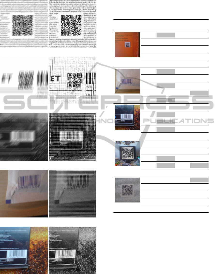
(a) Artificial blur. Angle: 22.5°, length: 25 pixels.
(b) Artificial blur. Angle: 74.5°, length: 70 pixels.
(c) Artificial blur. Angle: 40°, length: 50 pixels.
(d) Real blur. Angle: 63°, length: 16.52 pixels.
(e) Real blur. Angle: 156°, length: 11.38 pixels.
Figure 8: Images blurred by artificial ((a), (b), (c)) and real
((d), (e)) linear motion and their respective deconvolution
results.
Table 3: Comparison between the manual measuring and
the values determined by the algorithm for the 25 test im-
ages. Deviations of more than 5 pixels are highlighted.
angle angle length length
(manual) (algorithm) (manual) (algorithm)
100.0° 89.5° 14.22 px 14.63 px
180.0° 178.0° 17.96 px 18.29 px
38.0° 36.0° 34.13 px 36.57 px
90.0° 89.0° 21.79 px 22.26 px
32.0° 32.5° 26.95 px 28.44 px
150.0° 98.0° 11.38 px 11.38 px
90.0° 90.5° 25.6 px 25.6 px
42.0° 86.0° 8.46 px 9.31 px
1.0° 1.5° 20.9 px 85.33 px
63.0° 86.5° 16.0 px 16.52 px
91.0° 90.0° 9.23 px 46.55 px
7.0° 0.5° 15.28 px 8.53 px
156.0° 1.5° 11.38 px 11.38 px
62.0° 93.0° 10.04 px 11.64 px
59.0° 61.5° 14.42 px 14.22 px
178.0° 1.5° 14.22 px 14.63 px
91.0° 90.5° 15.75 px 15.06 px
12.0° 3.5° 6.4 px 4.92 px
140.0° 177.0° 14.03 px 4.92 px
171.0° 173.0° 8.83 px 8.83 px
179.0° 180.0° 9.23 px 20.48 px
174.0° 177.5° 15.28 px 18.96 px
75.0° 78.5° 8.53 px 2.67 px
142.0° 146.0° 14.42 px 14.63 px
45.0° 49.0° 14.63 px 15.52 px
recognised theoretically, this gives a rate of 8.1%.
Note, that even then the percentage of images on
which the reconstructed information is recognisable
with the naked eye is much higher. Obviously, the
scanning algorithm cannot handle the reconstructed
input images. This is most likely due to the additional
artefacts and diffuse edges caused by the deconvolu-
tion (Shan et al., 2008).
5.4 Performance
The algorithm has been implemented in Java in order
to conduct the experiments. It was first run on a stan-
dard desktop PC (3 GHz Intel Pentium D with 2 GB
IMAGAPP 2011 - International Conference on Imaging Theory and Applications
16

RAM) using JavaSE 1.6 and then ported to JavaME in
order to test it on a real mobile device. In the test run,
the whole process (preprocessing, blur parameter es-
timation and deconvolution) took about 500 ms for all
images to be completed on the desktop computer. The
exact same calculation took a total of about 22 sec-
onds on a last generation mobile device (Sony Erics-
son k800i), which is more than 40 times longer. While
some parts (e.g. the windowing) ran about 23 times
slower on the smartphone than on the desktop PC, the
FFT took 90 times as long. For the FFT the compar-
atively much slower floating point arithmetic makes
itself felt. However, note that next generation hard-
ware offers higher integer performance, much better
floating point support, and faster Java run time envi-
ronments. An analysis on the desktop computer re-
vealed that the FFT by far required the longest CPU
time (36%), followed by the Radon transform (18%)
and the calculation of the power spectrum (8%). Since
the complexity of the FFT is O(M log M), dependent
on the image size M, this also determines the com-
plexity of the deblurring algorithm as a whole.
6 CONCLUSIONS AND FUTURE
WORK
In this paper, a novel method combining and adapting
existing techniques for the estimation of motion blur
parameters and the subsequent removal of this blur is
presented. The algorithm is suitable for the execu-
tion on resource-constrained devices such as modern
smartphones and can be used as a preprocessing phase
for mobile information recognition software.
The algorithm uses the logarithmic power spec-
trum of a blurred image to identify the motion pa-
rameters. It introduces a new, specially adjusted
and therefore time-saving version of the Radon trans-
form for angle detection where features are only
sought after within a certain distance around the ori-
gin. The blur length is detected by analysing a one-
dimensional version of the spectrum. No cepstrum
and hence no further FFT are required. The estimated
parameters are then used to form a proper PSF with
which the blurred image can be deconvoluted. To do
so, a Wiener filter is employed.
It was found that the motion angle estimation
worked with a 5° accuracy for 92.71% of 330 arti-
ficially blurred images. The blur length determina-
tion delivered correct results with a maximum error
of 5 pixels in 95.73% of all cases. For images blurred
by real movement of an actual camera, these rates
amounted to roughly 60% and 88%, respectively. The
algorithm was implemented in Java to run on desk-
top computers as well as mobile devices. The algo-
rithm terminated within 500 ms on an standard desk-
top computer and took around 40 times longer on an
older smartphone. While sub second performance on
smartphones is not to be expected any time soon, exe-
cution time within a few seconds on modern hardware
should be attainable.
The application of the presented algorithm makes
some previously unrecognised barcodes to be recog-
nised by the ZXing decoder. However, the additional
artefacts caused by the deconvolution itself often hin-
ders the recognition in other cases. Yet, after the de-
convolution, completely blurred text become legible
again, and individual barcode features become clearly
distinguishable in many of the cases where decoding
failed. This gives reason to surmise that a success-
ful recognition might be possible if the decoders were
able to cope with the singularities of the reconstructed
images. Or, deconvolution methods that suppress the
emergence of artefacts could be explored.
REFERENCES
Burger, W. and Burge, M. J. (2008). Digital Image Pro-
cessing – An Algorithmic Introduction Using Java.
Springer.
Cannon, M. (1976). Blind deconvolution of spatially in-
variant image blurs with phase. Acoustics, Speech
and Signal Processing, IEEE Transactions on, 24(1),
pages 58–63.
Chalkov, S., Meshalkina, N., and Kim, C.-S. (2008).
Post-processing algorithm for reducing ringing arte-
facts in deblurred images. In The 23rd International
Technical Conference on Circuits/Systems, Computers
and Communications (ITC-CSCC 2008), pages 1193–
1196. School of Electrical Engineering, Korea Univer-
sity Seoul.
Chen, L., Yap, K.-H., and He, Y. (2007). Efficient recur-
sive multichannel blind image restoration. EURASIP
J. Appl. Signal Process., 2007(1).
Chu, C.-H., Yang, D.-N., and Chen, M.-S. (2007). Image
stabilization for 2d barcode in handheld devices. In
MULTIMEDIA ’07: Proceedings of the 15th Inter-
national Conference on Multimedia, pages 697–706,
New York, NY, USA. ACM.
Gonzalez, R. C. and Woods, R. E. (2008). Digital Image
Processing. Pearson Education Inc.
Harikumar, G. and Bresler, Y. (1999). Perfect blind restora-
tion of images blurred by multiple filters: Theory and
efficient algorithms. Image Processing, IEEE Trans-
actions on, 8(2), pages 202–219.
Krahmer, F., Lin, Y., McAdoo, B., Ott, K., Wang, J., Wide-
mann, D., and Wohlberg, B. (2006). Blind image de-
convolution: Motion blur estimation. Technical re-
port, University of Minnesota.
EFFICIENT MOTION DEBLURRING FOR INFORMATION RECOGNITION ON MOBILE DEVICES
17

Liu, Y., Yang, B., and Yang, J. (2008). Bar code recognition
in complex scenes by camera phones. In ICNC ’08:
Proceedings of the 2008 Fourth International Confer-
ence on Natural Computation, pages 462–466, Wash-
ington, DC, USA. IEEE Computer Society.
Lokhande, R., Arya, K. V., and Gupta, P. (2006). Identifi-
cation of parameters and restoration of motion blurred
images. In SAC ’06: Proceedings of the 2006 ACM
Symposium on Applied Computing, pages 301–305,
New York, NY, USA. ACM.
Otsu, N. (1979). A threshold selection method from gray-
level histograms. IEEE Transactions on Systems, Man
and Cybernetics, 9(1), pages 62–66.
Rekleitis, I. (1995). Visual motion estimation based on mo-
tion blur interpretation. Master’s thesis, School of
Computer Science, McGill University, Montreal.
Savakis, A. E. and Easton Jr., R. L. (1994). Blur identifica-
tion based on higher order spectral nulls. SPIE Image
Reconstruction and Restoration (2302).
Sezgin, M. and Sankur, B. (2004). Survey over image
thresholding techniques and quantitative performance
evaluation. Journal of Electronic Imaging, 13(1),
pages 146–168.
Shan, Q., Jia, J., and Agarwala, A. (2008). High-quality
motion deblurring from a single image. ACM Trans.
Graph., 27(3), pages 1–10.
Sorel, M. and Flusser, J. (2005). Blind restoration of images
blurred by complex camera motion and simultaneous
recovery of 3d scene structure. In Signal Processing
and Information Technology, 2005. Proceedings of the
Fifth IEEE International Symposium on, pages 737–
742.
Toft, P. (1996). The Radon Transform – Theory and Imple-
mentation. PhD thesis, Electronics Institute, Technical
University of Denmark.
Wang, Y., Huang, X., and Jia, P. (2009). Direction pa-
rameter identification of motion-blurred image based
on three second order frequency moments. Measur-
ing Technology and Mechatronics Automation, Inter-
national Conference on (1), pages 453–457.
White, J. and Rohrer, G. (1983). Image thresholding for op-
tical character recognition and other applications re-
quiring character image extraction. IBM J. Res. Dev,
27, pages 400–411.
Wiener, N. (1949). Extrapolation, Interpolation, and
Smoothing of Stationary Time Series. Wiley, New
York.
Wu, S., Lu, Z., Ping Ong, E., and Lin, W. (2007). Blind im-
age blur identification in cepstrum domain. In Com-
puter Communications and Networks, 2007. ICCCN
2007. Proceedings of 16th International Conference
on, pages 1166–1171.
Yitzhaky, Y. and Kopeika, N. (1996). Evaluation of the blur
parameters from motion blurred images. In Electrical
and Electronics Engineers in Israel, 1996., Nineteenth
Convention of, pages 216 –219.
IMAGAPP 2011 - International Conference on Imaging Theory and Applications
18
