
ANIMATION OF AIR BUBBLES WITH SPH
Markus Ihmsen, Julian Bader, Gizem Akinci and Matthias Teschner
Computer Science Department, University of Freiburg, Freiburg, Germany
Keywords:
Fluid Simulation, Smoothed Particle Hydrodynamics, Bubbles.
Abstract:
We present a physically-based multiphase model for simulating water and air bubbles with Smoothed
Particle Hydrodynamics (SPH). Since the high density ratio of air and water is problematic for existing
SPH solvers, we compute the density and pressure forces of both phases separately. The two-way coupling
is computed according to the velocity field. The proposed model is capable of simulating the complex
bubble flow, e. g. path instability, deformation and merging of bubbles and volume-dependent buoyancy.
Furthermore, we present a velocity-based heuristic for generating bubbles in regions where air is likely
trapped. Thereby, bubbles are generated on the fly, without explicitly simulating the air phase surrounding
the liquid. Instead of deleting the bubbles when they reach the surface, we employ a simple foam model. By
incorporating our model into the predictive-corrective SPH method, large time steps can be used. Thus, we can
simulate scenarios of high resolution where the size of the bubbles is small in comparison to the liquid volume.
1 INTRODUCTION
Air bubbles are a natural phenomenon that occurs in
everyday life. Whenever a liquid is poured into a
glass, bubbles are created by trapped air. Accord-
ingly, the visual realism of fluid animations is signif-
icantly enhanced by modeling the creation and flow
of bubbles. They might be even used to synthesize
the sound generated by the fluid (Moss et al., 2010).
However, the realistic simulation of air bubbles poses
some challenges.
In Computer Graphics, two major approaches are
employed for animating fluids, the Eulerian grid-
based method and the Lagrangian particle method.
While the Eulerian approach is particularly suited to
simulate large volumes of water, its performance is
limited by the grid spacing. In order to simulate small
scale features, a very fine resolution is required which
restricts the time step and increases the computing
time. In contrast, particle methods like Smoothed Par-
ticle Hydrodynamics (SPH) are suitable for capturing
small scale effects like the flow of tiny air bubbles.
In order to capture the creation of bubbles, the
computation of the air phase is required. However,
this invokes a significant computationaloverhead. For
grid-based methods, a second grid with fine resolution
is required which computes the air flow. In particle
methods, the air phase has to be represented explic-
itly.
In reality, air and water are interacting in a
two-way manner. Unlike water droplets, air bubbles
are under strong velocity diffusion because they are
coupled to the surrounding fluid by drag and lift
forces. According to the very large density ratio of
air to water (≈ 1000), water exerts a high pressure
on air bubbles which makes them merge rapidly.
As the bubbles grow, they rise faster due to the
rapid increase in buoyancy. In turn, those large and
fast rising bubbles significantly influence the liquid
flow. As stated in (Solenthaler and Pajarola, 2008),
modeling high density ratios with SPH is problematic
and may lead to numerical instabilities due to large
forces. Thus, the simulation of air bubbles is not
possible by directly employing the standard SPH
method (M¨uller et al., 2005; Solenthaler and Pajarola,
2008).
Contribution. We present a new SPH model for sim-
ulating air bubbles and foam. In order to handle the
high density ratio of air and water, we treat the two
phases separately. We account for the interaction of
the two phases by employing a drag force. As we
show, the proposed drag force is sufficient to capture
the two-way interaction realistically, while the numer-
225
Ihmsen M., Bader J., Akinci G. and Teschner M..
ANIMATION OF AIR BUBBLES WITH SPH.
DOI: 10.5220/0003322902250234
In Proceedings of the International Conference on Computer Graphics Theory and Applications (GRAPP-2011), pages 225-234
ISBN: 978-989-8425-45-4
Copyright
c
2011 SCITEPRESS (Science and Technology Publications, Lda.)
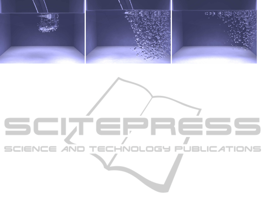
Figure 1: Trapped air. Air bubbles are generated on the fly in regions of high velocity differences. The bubble flow is
significantly influenced by the liquid. Bubbles are merging and deforming. This simulation contains 1.4 million liquid
particles and up to 6000 air particles.
ical stability is not affected.
We model the buoyancy of the air bubbles by
a saturated function that accounts for the volume.
Thereby, large bubbles rise faster than small bubbles.
Furthermore, a cohesion force is employed that mini-
mizes the surface and makes rising bubbles merge.
In order to simulate trapped air without explicitly
modeling the air surrounding the fluid, we generate
them on the fly in surface regions with high velocity
differences. When air particles have reached the sur-
face, they are treated as foam and finally deleted after
a user defined time.
The presented bubble model can be easily incor-
porated into any existing SPH solver with negligi-
ble computational overhead. We suggest to use the
predictive-corrective SPH (PCISPH) algorithm (So-
lenthaler and Pajarola, 2009) since it can handle large
time steps and is efficient to compute. Therefore, high
resolution scenes can be simulated where the size of
the bubbles is small in comparison to the liquid vol-
ume. A first example is illustrated in Fig. 1.
2 RELATED WORK
In this work, we focus on an SPH based fluid simu-
lation for animating air bubbles and their interaction
with water. In Computer Graphics, SPH is applied to
model different materials like gas (Stam and Fiume,
1995), deformable objects (Desbrun and Cani, 1996),
(Solenthaler et al., 2007), hair (Hadap and Magnenat-
Thalmann, 2001) and liquids (M¨uller et al., 2003).
However, the interaction of air and water is hardly
coveredsince the high density ratio poses severeprob-
lems to the SPH algorithm (Monaghan, 2002).
In (M¨uller et al., 2005), the standard SPH model
for single-phase fluid simulations (M¨uller et al., 2003)
is extended to handle multiple fluids. This approach
can handle density ratios of up to 10. In order to
simulate air bubbles, an artificial buoyancy force is
applied. However, as stated in (Solenthaler and Pa-
jarola, 2008), this approach suffers from falsified den-
sity estimations at the interface which induce wrong
pressure values. This in turn, limits the time step and
might result in numerical instabilities for fast rising
air particles due to large pressure forces. (Solen-
thaler and Pajarola, 2008) overcomes this problem by
ignoring the mass in the computation of the particle
density. Thereby, sharp density changes at the fluid
interface can be reproduced. Although this method
can handle density ratios of up to 100, the flow of
small, light volumes like air bubbles can not be re-
alistically handled. According to Solenthaler et al.,
the buoyant volumes can not break up the crystallized
particle configuration formed by the pressure forces.
In order to circumvent these problems, we ignore par-
ticle neighbors of other phases when computing the
density. Thus, we treat each phase separately. The in-
teraction of both phases is modeled via a drag force.
A similar idea is presented in (Cleary et al., 2007)
for simulating dynamic gas bubbles generated from
gas dissolution. In this approach, each phase is com-
puted separately, where the air bubbles are modeled
by discrete entities with fixed shape and the liquid is
computed with SPH. The bubbles are coupled to the
liquid via a drag force while the influence of the bub-
bles onto the liquid is neglected. In contrast, our bub-
ble model is based on SPH and the governing forces
are computed differently. Furthermore, we couple the
liquid and air phase in a two-way manner using a dif-
ferent formulation of the drag force.
Capturing the fine scale flow of bubbles with Eule-
rian methods, requires very fine grid resolutions. As
stated in (Hong et al., 2008), for numerical reasons,
each bubble should at least occupy 3 nodes in each di-
mension. Although, the computational overhead can
be minimized by adaptively refining the grid using an
octree (Losasso et al., 2004), the required grid spac-
ing significantly restricts the time step. Consequently,
pure grid-based methods like the regional level set
GRAPP 2011 - International Conference on Computer Graphics Theory and Applications
226

method (Zheng et al., 2006) are only suited to han-
dle relatively large bubbles in comparison to the fluid
volume. Alternatively, hybrid methods have been pro-
posed (Hong and Kim, 2003; Greenwood and House,
2004), in which the bubbles are simulated by passive
air particles that are advected according to the under-
lying grid. Similar to (K¨uck et al., 2002), the particles
are modeled as spheres which do no not change their
shape. By coupling the bubble particles to a low res-
olution grid, millions of air particles can be simulated
efficiently as shown in (Kim et al., 2010). However,
in these models the interaction of particles is often ne-
glected. Therefore, the size and shape of air bubbles
is not varying over time. In contrast, in the proposed
model, the air bubbles can consist of many particles.
The employed cohesion force minimizes the bubble
surface and makes bubbles merge. Since we recon-
struct the bubble surface from the particle positions
as described in (Solenthaler and Pajarola, 2008), the
bubble shape is deformable.
A hybrid solver is also proposed in (Hong et al.,
2008), where bubbles are simulated with SPH and
coupled to a grid-based fluid solver. The two phases
are coupled via the velocity field. However, due to
the insufficient resolution of the underlying grid, the
path instability of air bubbles can not be simulated by
this coupling. This is achieved by adapting the vor-
ticity confinement method (Fedkiw et al., 2001; Selle
et al., 2005) and artificial velocity disturbance based
on random numbers. In contrast, we model the liq-
uid phase with SPH. Thus, fine scale turbulences in
the liquid can be simulated. The proposed two-way
coupling is velocity based. Thereby, the bubble flow
is significantly influenced by the velocity field of the
liquid. Consequently, the path instability of bubbles
can be realistically simulated without adding artificial
disturbance.
In (Th¨urey et al., 2007), a two-dimensional shal-
low water model is coupled to a particle-based bub-
ble simulation. In order to capture three-dimensional
effects, the shallow water model makes a number of
simplifying assumptions. In particular, the fluid flow
is only modeled around bubbles and only if bubbles
are in the fluid. Thereby, the model is very efficient to
compute, but some effects can not be modeled, e. g.
inertia effects of the fluid. In contrast, the primary fo-
cus of the proposed model is not interactivity, but the
realism of the animation. However, we integrate our
model into the PCISPH algorithm presented in (So-
lenthaler and Pajarola, 2009). Thereby, large time
steps can be used which allows us to simulate mil-
lions of particles in reasonable time.
The remainder of the paper is organized as fol-
lows. First, we describe the basics of SPH and dis-
cuss its problems in handling high-density ratios. In
Sec. 4, the proposed model for simulating air bubbles
with SPH is explained in detail. Finally, we discuss
implementation issues and demonstrate the capability
of the presented method.
3 SPH
In this section, we briefly explain the basics of the
SPH method for single-phase and multiphase fluids.
3.1 Single-phase SPH
In SPH, the fluid is discretized into a finite set of par-
ticles i with position x
i
and velocity v
i
. Generally, a
particle quantity A
i
is approximatedby a smooth func-
tion which interpolates A
i
using a finite set of sam-
pling points j located within a distance h. This set of
sampling points is called particle neighborhood. The
smooth function is defined as
A
i
=
∑
j
m
j
ρ
j
A
j
W(x
i
− x
j
,h), (1)
where m
j
is the mass of j, ρ
j
its density and
W(x
i
− x
j
,h) is a kernel function with support radius
h.
The particle positions and velocities are integrated
according to internal and external forces. Internal
forces are viscosity, surface tension and pressure
forces, where the pressure force mainly governs the
macroscopic flow.
In Computer Graphics, two different algorithms
are generally used for computing the pressure of SPH
fluids, namely the state equation based algorithm
(SESPH) and the predictive-correctiveSPH algorithm
(PCISPH), see Alg. 1 and Sec. 4.4, respectively.
In SESPH, the pressure is related with the den-
sity. Commonly, for compressible fluids, the ideal
gas equation (2) (M¨uller et al., 2003) and for weakly-
compressible fluids, the Tait equation (3) (Monaghan,
1992; Becker and Teschner, 2007) are used
p
i
= c
2
s
(ρ
i
− ρ
0
) (2)
p
i
=
c
2
s
ρ
0
7
ρ
i
ρ
0
7
− 1
!
(3)
where c
s
denotes the speed of sound and ρ
0
the rest
density of the fluid. The density can be computed
with (1) as
ρ
i
=
∑
j
m
j
W(x
ij
,h) (4)
ANIMATION OF AIR BUBBLES WITH SPH
227

Algorithm 1: SESPH.
foreach particle i do
compute density (4) ;
compute pressure (3) or (2);
foreach particle i do
compute acceleration (8);
integrate position, velocity;
where x
ij
= x
i
− x
j
. The pressure force is directly
derived from the Navier-Stokes equations as
F
pressure
i
= −m
i
∑
j
m
j
p
i
ρ
2
i
+
p
j
ρ
2
j
!
∇W(x
ij
,h). (5)
According to (Monaghan, 2005), the viscosity
force for particle pairs with v
ij
· x
ij
< 0 is computed
as
F
viscosity
i
= m
i
∑
j
m
j
ν
v
ij
· x
ij
x
ij
2
+ εh
2
!
∇
i
W(x
ij
,h)
(6)
with the viscosity term ν = µ
2hc
s
ρ
i
+ρ
j
, where µ is the vis-
cosity constant.
The surface tension force can be elegantly com-
puted as proposed in (Becker and Teschner, 2007) as
F
sur face
i
= −k
s
∑
j
m
j
x
ij
W(x
ij
,h) (7)
where k
s
is a user-defined surface tension coefficient.
Finally, the acceleration a
i
of a particle i is com-
puted as
a
i
= m
−1
i
F
pressure
i
+ F
viscosity
i
+ F
sur face
i
+ g (8)
where g denotes the gravity. Similar to recent work
in the field of SPH, we use the above force equations
in conjunction with the cubic spline kernel of (Mon-
aghan, 1992). Alternative force equations and kernels
can be found in (M¨uller et al., 2003).
3.2 Multiphase SPH
The SESPH algorithm can be easily extended in or-
der to handle multiple fluids with different rest densi-
ties (M¨uller et al., 2005). However, as shown in (So-
lenthaler and Pajarola, 2008), miscible fluids with a
density ratio larger than 10 can not be realistically
simulated if the standard SPH density summation (4)
is used. The reason is that in SPH, the macroscopic
flow is mainly governed by the density computation.
Over- or underestimating the density leads to erro-
neous pressure values, which might result in unnat-
ural acceleration caused by erroneously introduced
pressure ratios. In (Solenthaler and Pajarola, 2008),
a different density model is proposed which treats
all particle neighbors as if they belong to the same
phase, i. e. have the same mass and rest density. This
model computes the density as ρ
i
= m
i
∑
j
W(x
ij
,h).
Thereby, the densities at the interface are computed
correctly.
Although this method can represent sharp den-
sity changes at the interface, it suffers from severe
limitations when dealing with large density ratios.
The buoyancy of small, light volumes is significantly
damped. As stated in (Solenthaler and Pajarola,
2008), this is due to the pressure force which com-
pels the particles to arrange in a stable lattice struc-
ture. This structure can not be broken by small vol-
umes like e. g. air bubbles.
In the following section, we present a new SPH
model for simulating the flow of air bubbles and the
two-way coupled interaction of air and water. The
presented model avoids the above mentioned prob-
lems.
4 BUBBLES
In order to simulate bubbles with SPH, we propose
to simulate the air and liquid phase separately, i. e.
only particle neighbors of the same phase contribute
to the density, pressure and general force computa-
tions. Accordingly, problems like e. g. high pressure
ratios or buoyancy dampening do not occur. We ac-
count for the interaction of both phases by employing
a new velocity based coupling.
In the following, we present force equations for
controlling the bubble flow and the interaction of both
phases. Subsequently, we propose an efficient method
for generating air bubbles caused by trapped air and
discuss a simple model for transforming air bubbles
into foam. Finally, we show how this model can be
integrated into the PCISPH algorithm.
4.1 Bubble Physics
In order to simulate bubbles realistically, we have to
capture the prominent effects of their complex behav-
ior. In general, bubbles have a sphere like shape ac-
cording to cohesion forces (surface and interface ten-
sion). However, since bubbles are heavily influenced
by the velocity field of the surrounding fluid, the bub-
ble shape is deforming. Furthermore, bubbles are dif-
ferent in size, where larger bubbles rise faster and at-
tract smaller bubbles.
For modeling these effects, we employ two forces
that are computed for the air phase only, namely
GRAPP 2011 - International Conference on Computer Graphics Theory and Applications
228
the buoyancy force F
buyoancy
and the cohesion force
F
cohesion
. The coupling of the two phases is realized
by the drag force F
drag
.
Buoyancy. The buoyancy force accelerates the air
bubble in direction of the liquid surface. In order to
make larger bubbles rise faster than smaller ones, the
buoyancy force should account for the volume of the
air bubble V
bub
. This leads to
F
buoyancy
i
= −k
b
·V
bub
· g (9)
where k
b
controls the buoyancy. However, computing
V
bub
is not straight forward without knowing which
particle belongs to which bubble. The determination
thereof invokes a significant computational overhead
which can be avoided by using a heuristic formula-
tion.
Replacing V
bub
in (9) with V
i
=
m
i
ρ
i
=
1
∑
j
W(x
ij
,h)
is
not suitable since V
i
gets smaller as the number of
neighbors grows, i. e. an isolated particle would rise
faster than a large bubble. On the other hand, cor-
relating the buoyancy with the density ρ
i
is also not
optimal since thereby, a compressed bubble (smaller
volume) would rise faster than an expanded one.
We therefore propose to relate the magnitude of
the buoyancy force to the number of particle neigh-
bors n with
F
buoyancy
i
= −m
i
k
b
·
k
max
− (k
max
− 1) · e
−0.1n
i
· g
(10)
where k
b
controls the minimum buoyancy and k
max
the maximum buoyancy. The mass is added to the
force formulation, in order to make the resulting
acceleration independent of the simulation resolu-
tion. Thus, the resulting acceleration caused by the
buoyancy force can be perfectly controlled since
kk
b
gk ≤
a
buoyancy
i
≤ kk
max
· k
b
· gk. This is also
illustrated in Fig. 2.
Cohesion. The coalescence of air bubbles is an im-
portant effect. Smaller air bubbles are attracted by
surrounding bubbles due to interface and surface ten-
sion forces. We model this behavior by employing an
artificial cohesion force
F
cohesion
i
= −k
c
m
i
∑
j
ρ
j
x
ij
(11)
where k
c
controls the strength of the cohesion force.
According to (11), air particles are attracted by neigh-
boring air particles with higher density. Thereby,
spatially close air bubbles do merge. Note that the
pressure force (5) counteracts the attraction, when the
density ρ
i
becomes too high. As a result, the surface
of the bubble is minimized while the forces converge
1
2
3
0 5 10 15 20 25 30
buoyancy scaling (times k
b
)
number of air neighbors
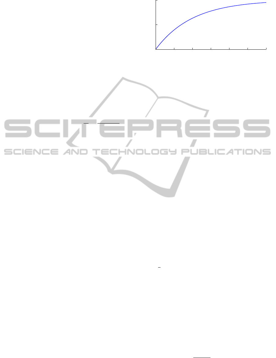
Figure 2: Scaling of the proposed volume-dependent buoy-
ancy for k
max
= 3. In order to account for the unknown
total bubble volume, the buoyancy of an air particle is non-
linearly related to its number of air neighbors.
to an equilibrium.
Two-way Coupling. In (Cleary et al., 2007)
and (Hong et al., 2008), the air phase is coupled to the
liquid phase via an empirical drag force. The effect
of the bubble momentum on the liquid phase is ne-
glected. With respect to the generally high Reynolds
number for air bubbles, the drag force F
drag
i
acting on
an air particle i is computed as
F
drag
i
= −k
d
A
bub
∑
liq
v
i
− v
liq
v
air
− v
liq
(12)
where k
d
is a constant drag coefficient, liq the liquid
neighbors of i and A
bub
is the surface area of the bub-
ble. Note that in (Cleary et al., 2007), air bubbles are
simulated as discrete spheres. Thus, A
bub
is easy to
compute. For the presented model, it is hard to com-
pute A
bub
since bubbles may have arbitrary shapes and
can consist of many particles.
In (12), the forces exerted by neighboring liquid
particles are related to the velocity difference, but the
flow direction and the distance of the particles are ne-
glected. Thus, a liquid neighbor j, that is very close
x
ij
≤
h
2
, influences the velocity of the air particle
by the same amount as a particle with distance h. Fur-
thermore, the partial drag force F
drag
ij
is non-zero as
long as
v
ij
> 0, whether the particles move towards
each other or not.
In contrast, we account for the distance and flow
direction (see Fig. 3). Therefore, we propose a drag
force that is motivated by the viscosity force (6) and
couples both phases in a two-way manner. Conse-
quently, the movement of the bubbles influences the
velocity field of the fluid and vice versa. The drag
force is defined as
F
drag
i
= m
i
∑
j
m
j
k
d
hc
s
ρ
i
+ ρ
j
Π
ij
∇
i
W(x
ij
,h) (13)
where k
d
denotes the drag constant. Π
ij
is zero
if either i and j belong to the same phase or if
ANIMATION OF AIR BUBBLES WITH SPH
229

Figure 3: Comparison of the proposed drag force (left) and
the drag force used in(Cleary et al., 2007) (right). The influ-
ence of the liquid particles (blue) onto the air particle (grey)
is shown. The velocity of the air particle is indicated by the
red arrow, the liquid is at rest. Partial forces are illustrated
by black arrows, while the resultant force is given by the
green arrow. The thickness denotes the magnitude.
v
ij
· x
ij
≤ 0, otherwise Π
ij
=
v
ij
·x
ij
k
x
ij
+εh
2
k
.
Acceleration. The acceleration of an air particle is
finally computed as
a
air
= m
−1
air
F
pressure
air
+ F
cohesion
air
+ F
buoyancy
air
+ F
drag
air
+g,
(14)
while for a liquid particle liq, the acceleration com-
putes to
a
liq
= m
−1
liq
F
pressure
liq
+ F
viscosity
liq
+ F
sur face
liq
+ F
drag
liq
+g.
(15)
Note that the proposed bubble model can be easily
integrated into any existing SPH solver. A discussion
is provided in Sec. 4.4, but first we suggest an heuris-
tic for generating and deleting air particles on the fly.
Thereby, trapped air can be simulated efficiently.
4.2 Trapped Air
Air bubbles are generated when air is trapped inside
the liquid. One possibility to capture this effect is to
simulate the air phase surrounding the liquid explic-
itly. In order to avoid the implied computational over-
head, we use a heuristic formulation in order to detect
regions where air is trapped.
The proposed heuristic is based on the following
observations:
• Air molecules are pulled inside the liquid by in-
flows
• The amount of trapped air grows with the velocity
of the inflow.
Accordingly, we generate air particles in sur-
face regions of high velocity differences. Therefore,
for each liquid particle on the surface, the magni-
tude of the velocity difference v
dif f
i
=
∑
j
m
j
ρ
j
(v
i
−
v
j
)W(x
ij
,h) is compared with a user defined thresh-
old v
t
. If
v
dif f
i
> v
t
, air is likely trapped at the po-
sition x
i
.
In order to relate the velocity of the inflow with
the volume of the generated air, two further conditions
must be met. First, the magnitude of the velocity must
be greater than a predefined threshold kv
i
k > v
min
.
Second, the number of air particle neighbors n
air
of
particle i should not be greater than
v
dif f
/v
t
. Con-
sequently, the number of generated particles grows
with the velocity of the inflow.
In summary, a liquid particle i generates
an air particle if
v
dif f
i
> v
t
, kv
i
k > v
min
and
n
air
<
v
dif f
/v
t
. The position and velocity of the
air particle are chosen to be the same as for the liquid
particle i.
Discussion. Our model computes the density and
pressure of the air and liquid phase separately. There-
fore, an air particle can be generated at the position
of a liquid particle without introducing high pressure
forces causing unnatural acceleration. This is in con-
trast to the multiphase methods presented in (M¨uller
et al., 2005; Solenthaler and Pajarola, 2008) where
high pressures are introduced when the distance of air
and liquid particles is too small. Thus, in these mod-
els, determining an appropriate position for a gener-
ated air particle without causing numerical instabili-
ties is not straightforward.
4.3 Foam
When air bubbles reach the liquid surface they do not
rise anymore, but float on the surface until they burst.
In reality, an air (foam) bubble disperses according
to film rupture in a two step process that can create
smaller bubbles. Note that the physics that govern this
complex behavior is not fully discovered yet (Bird
et al., 2010). However, for the purpose of animation,
we use a simplified model to simulate the floating and
bursting of foam bubbles.
First of all, we differentiate between particles that
are inside the liquid (rising bubbles) and particles that
are on the surface (foam). The liquid surface can be
determined either via a smoothed color field (M¨uller
et al., 2003; Keiser et al., 2005) or by comparing the
number of particle neighbors with a given threshold.
We treat an air particle i as on the surface (foam) ei-
ther if its density ρ
i
gets below a threshold t
ρ
or there
is no liquid neighbor j with (x
j
− x
i
) · g > 0.
The buoyancy force of foam particles is computed
as
F
buoyancy
i
= −m
i
g (16)
GRAPP 2011 - International Conference on Computer Graphics Theory and Applications
230
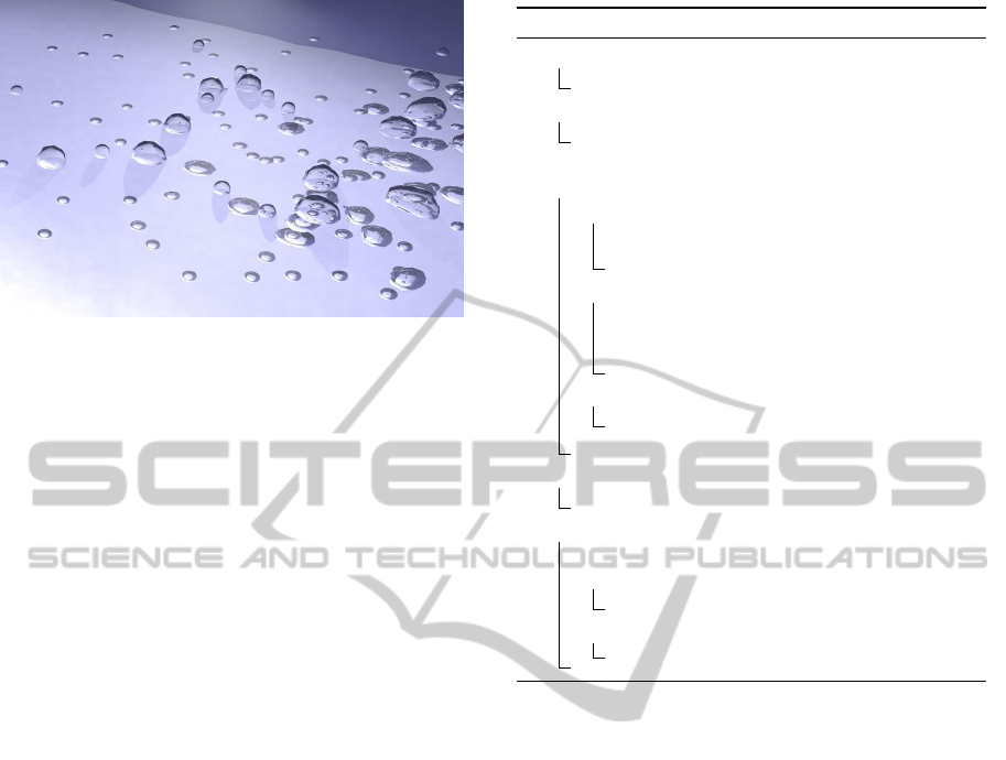
Figure 4: Foam bubbles. Air particles are not directly
deleted when they reach the surface, but treated as foam.
They float on the surface, according to the buoyancy and
drag force. Due to the cohesion force, foam bubbles are
different in size and shape.
This force cancels out the acceleration due to gravity
g. Like rising bubble particles, foam particles are
coupled to the liquid by the drag force (13). Thereby,
the resulting velocity of foam particles is governed
by the surrounding liquid. Thus, the foam floats
on the liquid surface. Due to the cohesion force,
foam particles also cluster on the surface, trying to
minimize the surface. Consequently, foam bubbles
are different in size and shape (see Fig. 4).
Deletion of Foam Particles. When an air particle
reaches the surface it is given a floating time t
f
, i. e.
time until the particle is deleted. In order to improve
the realism, we vary t
f
for each particle randomly us-
ing a uniform distribution. However, if two foam par-
ticles merge, i. e. are neighbors, the minimum of their
floating times is assigned to both particles. Thereby,
foam bubbles consisting of more than one particle dis-
perse at once.
4.4 Algorithm
In order to simulate water realistically, the compress-
ibility should be set very low. In SESPH, the com-
pressibility is controlled by the speed of sound (see
(2), (3)). Setting c
s
higher reduces the compressibil-
ity, but also restricts the time step. In (Solenthaler
and Pajarola, 2009), an alternative SPH algorithm for
incompressible fluids is suggested, called PCISPH.
In this approach, the compression error is predicted
and corrected iteratively. Thereby, significantly larger
time steps can be used, while the computational over-
head is small compared to SESPH. Accordingly, high-
resolution fluids can be simulated within reasonable
time.
The proposed bubble model can be directly incor-
Algorithm 2: PCISPH with bubbles.
foreach air particle do
compute forces (11), (10), (13), (16);
foreach liquid particle do
compute forces (6), (7), (13) ;
k = 0 ;
while (max(ρ
∗
err
) > η or k < 3) do
forall particles do
predict velocity ;
predict position ;
forall particles do
update distances to neighbors;
predict density variation;
update pressure ;
forall particles do
compute pressure force;
k+ = 1;
forall particles do
compute acceleration (14) or (15);
forall particles i do
integrate velocity and position;
if i is liquid then
test for air generation
else
test for deletion
porated into the PCISPH algorithm (see Alg. 2) with
negligible computational overhead. Furthermore, the
time step is not affected by the high density ratio of
water and air. This is due to the velocity based cou-
pling which avoids the computation of the pressure
forces at the water-air interface.
Explaining the prediction and correction loop of
the PCISPH algorithm is beyond the scope of this pa-
per. Detailed explanations can be found in (Solen-
thaler and Pajarola, 2009; Ihmsen et al., 2010).
5 RESULTS
In this section, we briefly cover implementation as-
pects and parameter settings. Then, we demonstrate
the capability of the proposed model to animate the
air bubbles and their interaction with water.
Implementation. In order to correct the density
at the fluid surface, we use the constant correction
technique as described in (Bonet and Kulasegaram,
2002). Positions and velocities are updated using
the Euler-Cromer scheme. The neighborhood search
is computed using the parallelized compact hashing
ANIMATION OF AIR BUBBLES WITH SPH
231

method (Ihmsen et al., 2011).
The surfaces are extracted by first mapping the
particle positions to a scalar field as described in (So-
lenthaler et al., 2007) and then using the Marching
Cubes algorithm (Lorensen and Cline, 1987). The
resulting meshes are rendered with POV-Ray.
Parameter Setting. In all our 3D scenes, we set the
reference density of water to 1000 kg/m
3
and for air
particles we set it to 1 kg/m
3
. The particle mass is
computed as ρ
0
/(0.5h)
3
, where 0.5h is the initial par-
ticle spacing, which is 0.02 in most of our scenes. The
gravity is set to (0, −9.81,0)
T
. Velocities and accel-
erations are given in m/s, m/s
2
respectively.
For the bubbles, we empirically found the follow-
ing setting to obtain good results: the buoyancy coef-
ficients k
b
= 14 and k
max
= 6, cohesion k
c
= 12 and
the drag coefficient k
d
is set to 8 for air particles and
to 3 for water. We have varied the parameters for gen-
erating air bubbles in order to show their effect on the
simulation (see Sec. 5.2).
Note that the coefficients introduced for the bub-
ble model are independent of the resolution h. By
increasing the parameters k
d
,k
c
and k
b
, the effect of
the corresponding force is amplified.
5.1 Bubble Flow
The basic capability of the presented bubble model
is demonstrated by simulating rising bubbles in calm
water (see Fig. 5). In this example scene, air particles
are randomly seeded at the bottom. The initial fluid
velocity is zero. According to the proposed two-way
coupling, the velocity field of the fluid is influenced
by the air phase and vice versa. Thereby, small scale
turbulences are generated which results in a natural
zig-zag flow of the bubbles without adding random
disturbance. As the example shows, the prominent
effects of air bubble flow can be successfully cap-
tured, e. g. merging, path instability, volume depen-
dent buoyancy.
In this scene, 2.4 million water particles and up to
10k air particles are simulated. The time step is set
to 0.0015s which guarantees a compressibility of less
than 1.5%.
5.2 Bubble Generation
A major contribution of the presented model is the
generation of air bubbles. In contrast to existing work,
air is generated in surface regions with high local ve-
locity differences. According to the velocity based
coupling, bubbles can be generated on the fly without
Figure 5: Rising bubbles in calm water. Bubbles are differ-
ent in shape and size due to the cohesion force.
causing numerical instabilities. The generation of air
bubbles is demonstrated in two example scenes.
In the first example, an inflow is simulated that
is poured into a volume of water (see Fig. 1). High
velocity differences occur around the inflow. Accord-
ingly, air particles are generated. Although, the bub-
ble flow is mainly influenced by the turbulent velocity
field of the liquid, the individual flow is quite differ-
ent. Bubbles are varying in size and shape according
to the cohesion force. Due to the volume dependent
buoyancy, larger bubbles rise faster and more straight,
while smaller bubbles are mainly influenced by the
liquid. According to the proposed foam model, the air
bubbles float realistically on the surface before they
burst. For this example, we set the average floating
time t
f
to 0.7s. In this example, a liquid surface par-
ticle only generates an air particle if the velocity dif-
ference is larger than v
t
= 0.3 and the magnitude of
its velocity is larger than v
min
= 3. Note that less air
would be generated if v
t
or v
min
are set higher.
The second example demonstrates that the amount
of generated air particles scales with the magnitude
of the velocity difference. Therefore, three underwa-
ter inflows are simulated (see Fig. 6). The veloci-
ties v
n
= (x
n
,0,0)
T
of the water inflows are set dif-
ferently, where x
1
= 5.5, x
2
= 7.0 and x
3
= 9.0. v
t
is set to 0.75 and v
min
to 3.5. Thereby, the veloc-
ity differences around the inflow do vary. According
to the proposed heuristic (see Sec. 5.2), most of the
air particles are generated by the fastest inflow, while
the slowest inflow generates significantly less bub-
bles. Furthermore, higher inflow velocities result in
larger turbulences. Since these vorticities are mapped
onto the bubble flow, the bubbles indicate the liquid
flow. Note that without the animation of bubbles, the
liquid inflow would not be visible in this example.
Again, spatially close air particles merge. Con-
sequently, some air bubbles get quite large, particu-
larly for the fast inflow. These large bubbles rise very
fast due to the volume dependent buoyancy force. Ac-
cording to the drag force, they significantly influence
GRAPP 2011 - International Conference on Computer Graphics Theory and Applications
232
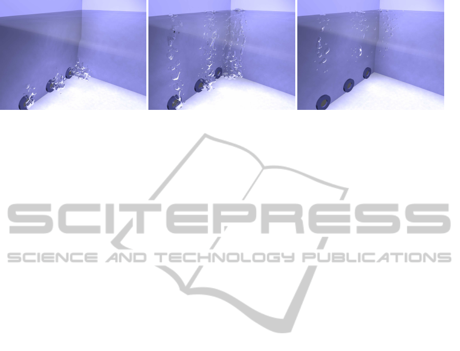
Figure 6: Underwater inflows. Water streams out of the three pipes with different velocities. The inflow in front has the lowest
velocity and the inflow in the back the highest. Note that the amount of generated air scales with the velocity of the inflow.
Larger air bubbles influence the liquid significantly. The simulation uses 650k water particles and up to 2k air particles.
the liquid, as is clearly visible at the liquid surface. In
both scenes, we set the time step to 0.002s.
6 CONCLUSIONS
We have presented a new air bubble model for SPH.
Numerical instabilities, invoked by the high density
ratio at the bubbles interface, are avoided by coupling
the two phases via the velocity field. Since the
coupling is in both directions, small scale turbulences
are naturally captured, e. g. path instability. In
contrast to existing models, the bubbles are simulated
with SPH and not just by solid spheres. According
to the proposed cohesion force, effects like merging
and deformation of bubbles can be successfully
simulated. Furthermore, we have proposed a ve-
locity based heuristic that generates air bubbles for
inflows. Thereby, trapped air is animated efficiently,
i.e. without explicitly simulating the air phase
surrounding the liquid. We also employ a simple
foam model in order to simulate floating air bubbles.
By incorporating the bubble model into the PCISPH
method, large time steps can be used. This allows
to simulate high-resolution animations where the
bubbles are small in size in comparison to the liquid
volume. This is demonstrated in the example scenes.
Future Work. In this work, we do not cover the in-
teraction of air bubbles with rigid or deformable bod-
ies. Effects like natural surface attraction of bubbles
to solid surfaces would certainly further improve the
realism of the simulation.
Moreover, we think that the performance can be
further improved by using smaller support radii for
air particles than for liquid particles. This is proposed
for single-phase fluids in (Desbrun and Cani, 1996),
(Adams et al., 2007). In scenarios, where the influ-
ence of air bubbles onto water can be neglected, the
air bubble model can be applied as a post-processing
step. The generation of bubbles and their flow can
be sufficiently computed using the already simulated
velocity field of the liquid. This could be interest-
ing for highly turbulent fluid simulations like rivers
or waves.
ACKNOWLEDGEMENTS
This project is supported by the German Research
Foundation (DFG) under contract number TE 632/1-
1.
REFERENCES
Adams, B., Pauly, M., Keiser, R., and Guibas, L. (2007).
Adaptively sampled particle fluids. In SIGGRAPH
’07: ACM SIGGRAPH 2007 papers, page 48, New
York, USA. ACM Press.
Becker, M. and Teschner, M. (2007). Weakly compress-
ible SPH for free surface flows. In SCA ’07: Pro-
ceedings of the 2007 ACM SIGGRAPH/Eurographics
symposium on Computer animation, pages 209–217,
Aire-la-Ville, Switzerland. Eurographics Association.
Bird, J. C., de Ruiter, R., Corbin, L., and Stone, H. A.
(2010). Daughter bubble cascades produced by fold-
ing of ruptured thin films. Nature, 465:759–762.
Bonet, J. and Kulasegaram, S. (2002). A simplified ap-
proach to enhance the performance of smooth particle
hydrodynamics methods. Applied Mathematics and
Computation, 126(2-3):133–155.
Cleary, P., Pyo, S., Prakash, M., and Koo, B. (2007).
Bubbling and frothing liquids. ACM Transaction on
Graphics, 26(3):97.
Desbrun, M. and Cani, M.-P. (1996). Smoothed Particles: A
new paradigm for animating highly deformable bod-
ies. In Eurographics Workshop on Computer Anima-
tion and Simulation (EGCAS), pages 61–76. Springer-
Verlag.
Fedkiw, R., Stam, J., and Jensen, H. (2001). Visual sim-
ulation of smoke. In SIGGRAPH ’01: Proceedings
ANIMATION OF AIR BUBBLES WITH SPH
233

of the 28th annual conference on Computer graphics
and interactive techniques, pages 15–22, New York,
USA. ACM.
Greenwood, S. T. and House, D. H. (2004). Better with
bubbles: enhancing the visual realism of simulated
fluid. In SCA ’04: Proceedings of the 2004 ACM SIG-
GRAPH/Eurographics symposium on Computer an-
imation, pages 287–296, Aire-la-Ville, Switzerland.
Eurographics Association.
Hadap, S. and Magnenat-Thalmann, N. (2001). Modeling
Dynamic Hair as a Continuum. Computer Graphics
Forum, 20(3):329–338.
Hong, J.-M. and Kim, C.-H. (2003). Animation of Bubbles
in Liquid. Computer Graphics Forum, 22:253–262.
Hong, J.-M., Lee, H.-Y., Yoon, J.-C., and Kim, C.-H.
(2008). Bubbles Alive. In SIGGRAPH ’08: ACMSIG-
GRAPH 2008 papers, pages 1–4, New York, USA.
ACM.
Ihmsen, M., Akinci, N., Becker, M., and Teschner, M.
(2011). A Parallel SPH Implementation on Multi-core
CPUs. Computer Graphics Forum. to appear.
Ihmsen, M., Akinci, N., Gissler, M., and Teschner, M.
(2010). Boundary Handling and Adaptive Time-
stepping for PCISPH. In Proc. VRIPHYS, pages 79–
88.
Keiser, R., Adams, B., Gasser, D., Bazzi, P., Dutr´e, P., and
Gross, M. (2005). A Unified Lagrangian Approach to
Solid-Fluid Animation. In Proceedings of the Euro-
graphics Symposium on Point-Based Graphics, pages
125–134.
Kim, D., Song, O.-Y., and Ko, H.-S. (2010). A practical
simulation of dispersed bubble flow. In ACM SIG-
GRAPH 2010 papers, SIGGRAPH ’10, pages 70:1–
70:5, New York, USA. ACM.
K¨uck, H., Vogelgsang, C., and Greiner, G. (2002). Simula-
tion and rendering of liquid foams. In In Proc. Graph-
ics Interface 02 (2002), pages 81–88.
Lorensen, W. and Cline, H. (1987). Marching cubes: A
high resolution 3D surface construction algorithm. In
SIGGRAPH ’87: Proceedings of the 14th annual con-
ference on Computer graphics and interactive tech-
niques, pages 163–169, New York, USA. ACM Press.
Losasso, F., Gibou, F., and Fedkiw, R. (2004). Simulating
water and smoke with an octree data structure. In SIG-
GRAPH ’04: ACM SIGGRAPH 2004 Papers, pages
457–462, New York, USA. ACM.
Monaghan, J. (1992). Smoothed particle hydrodynamics.
Ann. Rev. Astron. Astrophys., 30:543–574.
Monaghan, J. (2002). SPH compressible turbulence.
Monthly Notices of the Royal Astronomical Society,
335(3):843–852.
Monaghan, J. (2005). Smoothed particle hydrodynamics.
Reports on Progress in Physics, 68(8):1703–1759.
Moss, W., Yeh, H., Hong, J.-M., Lin, M. C., and Manocha,
D. (2010). Sounding liquids: Automatic sound syn-
thesis from fluid simulation. ACM Trans. Graph.,
29(3):1–13.
M¨uller, M., Charypar, D., and Gross, M. (2003). Particle-
based fluid simulation for interactive applications.
In SCA ’03: Proceedings of the 2003 ACM SIG-
GRAPH/Eurographics symposium on Computer an-
imation, pages 154–159, Aire-la-Ville, Switzerland.
Eurographics Association.
M¨uller, M., Solenthaler, B., Keiser, R., and Gross, M.
(2005). Particle-based fluid-fluid interaction. In
SCA ’05: Proceedings of the 2005 ACM SIG-
GRAPH/Eurographics symposium on Computer ani-
mation, pages 237–244, New York, USA. ACM.
Selle, A., Rasmussen, N., and Fedkiw, R. (2005). A vor-
tex particle method for smoke, water and explosions.
In SIGGRAPH ’05: ACM SIGGRAPH 2005 Papers,
pages 910–914, New York, NY, USA. ACM.
Solenthaler, B. and Pajarola, R. (2008). Density Contrast
SPH Interfaces. In SCA ’08: Proceedings of the 2008
ACM SIGGRAPH/Eurographics Symposium on Com-
puter Animation, pages 211–218.
Solenthaler, B. and Pajarola, R. (2009). Predictive-
corrective incompressible SPH. In SIGGRAPH ’09:
ACM SIGGRAPH 2009 Papers, pages 1–6, New York,
USA. ACM.
Solenthaler, B., Schl¨afli, J., and Pajarola, R. (2007). A uni-
fied particle model for fluid-solid interactions. Com-
puter Animation and Virtual Worlds, 18(1):69–82.
Stam, J. and Fiume, E. (1995). Depicting fire and other
gaseous phenomena using diffusion processes. In
SIGGRAPH ’95: Proceedings of the 22nd annual con-
ference on Computer graphics and interactive tech-
niques, pages 129–136, New York, USA. ACM Press.
Th¨urey, N., Sadlo, F., Schirm, S., M¨uller-Fischer, M., and
Gross, M. (2007). Real-time simulations of bub-
bles and foam within a shallow water framework.
In SCA ’07: Proceedings of the 2007 ACM SIG-
GRAPH/Eurographics symposium on Computer an-
imation, pages 191–198, Aire-la-Ville, Switzerland.
Eurographics Association.
Zheng, W., Yong, J.-H., and Paul, J.-C. (2006). Simu-
lation of bubbles. In SCA ’06: Proceedings of the
2006 ACM SIGGRAPH/Eurographics symposium on
Computer animation, pages 325–333, Aire-la-Ville,
Switzerland. Eurographics Association.
GRAPP 2011 - International Conference on Computer Graphics Theory and Applications
234
