
PRODUCING AUTOMATED MOSAIC ART IMAGES OF HIGH
QUALITY WITH RESTRICTED AND LIMITED COLOR
PALETTES
Tefen Lin and Jie Wang
Department of Computer Science, University of Massachusetts, Lowell, MA 01854, U.S.A.
Keywords: Error diffusion, Floyd-Steinberg dither, Serpentine Floyd-Steinberg, Block error diffusion, Sub-block error
diffusion.
Abstract: In mosaic art images made from bricks, tiles, or counted cross-stitch patterns, artists would need to divide
the original image into small parts of reasonable sizes and shapes and represent the colors of each part using
just one “closest” color selected from a given color palette. Using standard methods to automate this
process, the resulting mosaic image may contain undesirable visual artifacts of patches and color bandings.
Error-diffusion dithering algorithms have been used to reduce such artifacts. We observe that image parsing
directions are critical for diffusing errors, and we present a new error-diffusion scheme called “Four-Way
Block dithering” (FWB) to correct certain artifacts caused by existing methods, including the directional
and latticed appearance produced by Floyd and Steinberg’s dithering (FSD). FWB divides the input image
into blocks of equal size with each block consisting of four sub-blocks such that the size of each sub-block
is suitable for an underlying error-diffusion algorithm. Scanning the blocks from left to right and from top to
bottom, for each block being scanned, FWB starts from the center of the block and diffuses errors along
four directions on each sub-block. We show that FWB can better retain the original structure and reduce
unstructured artifacts. We also show that FWB dithering produces much better peak signal-to-noise ratios
on mosaic images over those generated by FSD.
1 INTRODUCTION
Photographic images are used widely in digital forms.
Uploading self portraits or other images to blogs, for
example, has become a common practice. As an
application of digitized images, we have worked with
brick and tile companies during the past several years
to develop a web-based system that creates automated
mosaic art images with small pieces of colored tiles or
bricks. Based on current technology, tile
manufacturers can only produce tiles of limited
colors. In particular, the tile manufacturers we have
worked with can typically produce 48 different colors
on square tiles of small size, which can be as small as
½ cm × ½ cm. These 48 colors form our color palette
(see Figure 1). We chose to work on 1 cm × 1 cm
square tiles for the purpose of reducing manufacturing
cost and easing the labor on assembling the pieces
together. We also need to resize the original image to
fit in standard picture frames. A typical picture frame
is 50 cm wide with its height determined by the
width/height ratio of the original image.
Our process can be described as follows: We first
resize the original image of size w × h pixels to the
desired size of w’ pixels wide and w’h/w pixels high,
where w represents width and h represents height. For
example, the original image of da Vinci’s painting of
Mona Lisa (the portion of the head) is 136 × 182
pixels. We resize it by retrieving its own embedded
thumbnail and scale it to the size 50 × 64 pixels (see
Figure 2 (a)). If the image does not contain an
embedded thumbnail image, we create a thumbnail
image to size 50 × 64 pixels by scaling the main image.
This resized image is referred to as the input image.
Most of the colors in the input image may be
unavailable in the given color palette.
Figure 1: The color palette available for tiles.
125
Lin T. and Wang J..
PRODUCING AUTOMATED MOSAIC ART IMAGES OF HIGH QUALITY WITH RESTRICTED AND LIMITED COLOR PALETTES.
DOI: 10.5220/0003326601250133
In Proceedings of the International Conference on Imaging Theory and Applications and International Conference on Information Visualization Theory
and Applications (IMAGAPP-2011), pages 125-133
ISBN: 978-989-8425-46-1
Copyright
c
2011 SCITEPRESS (Science and Technology Publications, Lda.)

Next, for each pixel in the input image, we
calculate the Euclidean distance from its RGB value to
the RGB value of each of the 48 available colors in the
color palette (note that each RGB value may be
viewed as a 3-dimensional vector), and select a color
with the smallest Euclidean distance. If there is more
than one color with the same smallest distance, we
select one from these colors with the smallest
Euclidean distance from their HSB (Hue, Saturation,
and Brightness) values to the HSB value of the pixel.
Figure 2 (b) shows the result of this process.
(a) (b) (c)
Figure 2: Size of these images: 50 pixels wide and 67 pixels
high. (a) Input image. (b) The image with reduced color
using the limited color palette. (c) The image produced by
Floyd-Steinberg dither .
This process is likely to yield color bandings and
patches that produce dramatically different visual
effect from the input image (as shown in Figure 2 (b))
because of color reduction. To enhance the visual
quality of the image, we need to find ways to conceal
or minimize these artifacts. This process is referred to
as color quantization.
Dithering is a useful technique to transform an
image of continuous tone to an image of limited given
colors. A number of dithering algorithms have been
devised during the past three decades, including
threshold dithering, random dithering, pattern
dithering, and error-diffusion dithering. Error
diffusion dithering intends to diffuse the quantization
error of a given pixel to its neighboring pixels.
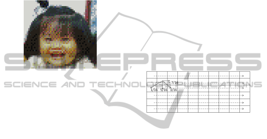
Published in 1975, Floyd and Steinberg’s error
diffusion dithering algorithm (Floyd and Steinberg,
1975), referred to as FSD, has been the most popular
dithering algorithm. It uses a set of values of 1/16,
5/16, 3/16, and 7/16 to diffuse a pixel’s error to its
lower left, lower, lower right, and right neighbors,
respectively, producing a dithering image shown in
Figure 2 (c).
Listed below are a number of other error-diffusion
methods.
Coefficient error diffusion dithering. Jarvis,
Judice, and Nink (
Judice and Ninke, 1976
) devised a
dithering algorithm using a much more complex
error diffusion coefficient matrix than the one used in
FSD. Shiau and Fan’s dithering algorithms (
Shiau and
Fan, 1993
), Stucki’s dithering algorithm (
Stucki, 1981
),
Burkes’ dithering algorithm (
Daniel Burkes, 1988
), and
Atkinson’s dithering algorithm (
Atkinson, 2003)
all
use different sets of error diffusion coefficient
matrices.
Changing image parsing direction. Dithering is
often carried out by scanning a pixel one at a time,
from left to right and from top to bottom. Other
parsing directions may be applied. For example, one
may parse an image following a serpentine path
using the FSD error diffusion coefficient matrix,
instead of parsing it line by line or with a space-
filling curve (
Riemersma, 1998
).
Variable coefficients error diffusion.
Ostromoukhov (
Ostromoukhov, 2001
) proposes to use
variable error diffusion coefficent matrix based on
the input image.
Block error diffusion and sub-block error
diffusion. Both algorithms parse image four pixels at
a time, which were proposed by Damera-Venkata
and Evans (
Damera-Venkata and Evans, 2001
),
respectively. The sub-block error diffusion improves
block error diffusion, using four 2 × 2 error diffusion
matrices for pixels contained in one block.
Reported in (Caca Labs., 2010), the serpentine
dithering, block dithering, and sub-block dithering
tend to produce poorer image quality than FSD.
Hocevar and Niger (Hocevar and Niger, 2008)
confirmed that the original FSD coefficients were
indeed amongst the best possible for raster scan.
However, as observed by others and confirmed by
our studies, FSD still contains a number of
drawbacks. For example, FSD tends to produce
noticeable visually distributing artifacts in highlight
and dark areas. More ever, on certain intensity levels
close to ½, 1/3, 2/3, ¼, and ¾, patches of regular
structure are likely to appear. Uneven transitions
between “structure” and unstructured” areas may be
clearly visible (Ostromoukhov, 2001).For example,
as shown in Figure 2 (c), Mona Lisa’s right eye
displays a serious defect—it is much narrower than
that shown in Figure 2 (a) and (b), which makes the
right eye look like half closed.
FSD parses an image in raster scan. Observed by
Hocevar and Niger (Hocevar and Niger, 2008) and
confirmed by our experiments, errors in FSD tend to
propagate to the lower-left direction of each pixel or
to the lower-right direction. Thus, the output image
may look tilted. We observe from a large number of
imaging experiments that the image parsing direction
is crucial in error diffusion. This is probably due to
the fact that, once a pixel completely diffuses
IMAGAPP 2011 - International Conference on Imaging Theory and Applications
126
quantization error to its neighbors, only one direction
of the quantization error would be nicely diffused,
but not the errors in other directions. This effect
seriously affects the image quality and causes the
output image to appear directional and latticed. For
example, Figure 3 produced by FSD clearly depicts
the vertical directions and lattice appearance. More
explanations why this could happen will be presented
in Section 3.
Figure 3: An image produced by FSD clearly depicts
vertical directions and lattice appearance. Size of the
output image: 50 pixels wide and 47 pixels high.
To retain the original image structure and resolve
the directional and latticed appearance, we device a
new error diffusion scheme called Four-Way Block
(FWB) diffusion. FWB divides the input image into
blocks of equal size with each block consisting of
four sub-blocks such that the size of each sub-block
is suitable for an underlying error-diffusion algorithm.
For example, when we use FSD, the size of sub-
blocks may be set to 3k pixels wide and 2k pixels
high for the same positive integer k. Scanning blocks
from left to right and from top to bottom, for each
block being scanned, FWB starts from the center of
the block and diffuses errors along four directions on
each sub-block. This process has the effect of
diffusing errors backward. This is different from the
existing error-diffusion dithering methods that
always move and diffuse errors forward in the
direction it parses the image. This mechanism helps
to diffuse errors without leaving a visible trace of
error propagation. We show that FWB can improve
the quality of mosaic images. In particular, we show
that FWB produces much better peak signal-to-noise
ratios (PSNR) on mosaic images over those
generated by FSD.
The rest of the paper is organized as follows. In
Section 2 we will briefly describe the FSD algorithm.
We present our new FWB error-diffusion scheme in
Section 3 and provide detailed dissemination. In
Section 4 we provide running comparisons of FSD
and FWB using FSD as the underlying error-
diffusion algorithm. We conclude the paper in
Section 5. In Appendix we provide a number of
examples of mosaic art images.
2 FLOYD-STEINBERG ERROR
DIFFUSION DITHERING
FSD is widely used in dithering images of continuous
tone. The quantization error, which is the difference
between the color in the input image and the closest
color in the limited color palette, will be distributed to
its four neighboring pixels by the coefficient error
diffusion matrix shown in (1). FSD scans the original
image from left to right and from top to bottom as
shown in Figure 4.
1/16 *
000
0
7
153
(1)
Figure 4: Floyd-Steinberg dithering scans an image file
from top to bottom and from left to right one pixel at a time.
Each cell in the Figure represents one pixel.
3 FWB, A NEW SCHEME FOR
ERROR DIFFUSION
How to reduce artifacts caused by FSD is a central
issue in generating automated mosaic art images. We
devise FWB based on the following three
observations.
1. FSD has a simple parsing mechanism based on a
nice error-diffusion coefficient matrix. Other
error-diffusion algorithms may also work nicely
for certain type of images.
2. The image parsing direction is crucial in error
diffusion.
3. The existing error diffusion algorithms only
diffuse errors in a forward direction. We note that
making diffusion backward may help diffuse
errors better.
The FWB error-diffusion scheme follows the
following four steps:
PRODUCING AUTOMATED MOSAIC ART IMAGES OF HIGH QUALITY WITH RESTRICTED AND LIMITED
COLOR PALETTES
127
1. Choose an underlying error-diffusion algorithm
(FSD, for example).
2. Divide a given input image to blocks of equal
size with each block consisting of four sub-
blocks of equal size (except the bottom and right-
hand edges) suitable for the underlying error-
diffusion algorithm. For example, when FSD is
chosen, we may set the sub-block size to be 3k
pixels wide and 2k pixels height for some
positive integer k.
3. Scan the blocks from left-to-right and from top to
bottom. For each block being scanned, apply the
underlying error-diffusion algorithm in four
directions on each sub-block starting from the
center point of the block. If a block is already
parsed, then it does not allow its neighboring
blocks to rewrite its values.
4. Use both Euclidean distances of RBG and HSV
values to select the closest color from the given
color palette for the output pixel.
Note that FWB may not be able to divide a given
image evenly, that is, if we divide the image starting
from the upper-left pixel, then, we may not be able to
obtain full blocks at the bottom or at the right-hand
side. When this happens, we will just apply the
underlying error-diffusion algorithm on these blocks
in the usual manner. This is a small price to pay, and
the majority of the pixels will receive better error
diffusion.
Denote by FWB-XYZ the FWB scheme with
XYZ being the name of the underlying error-diffusion
algorithm.
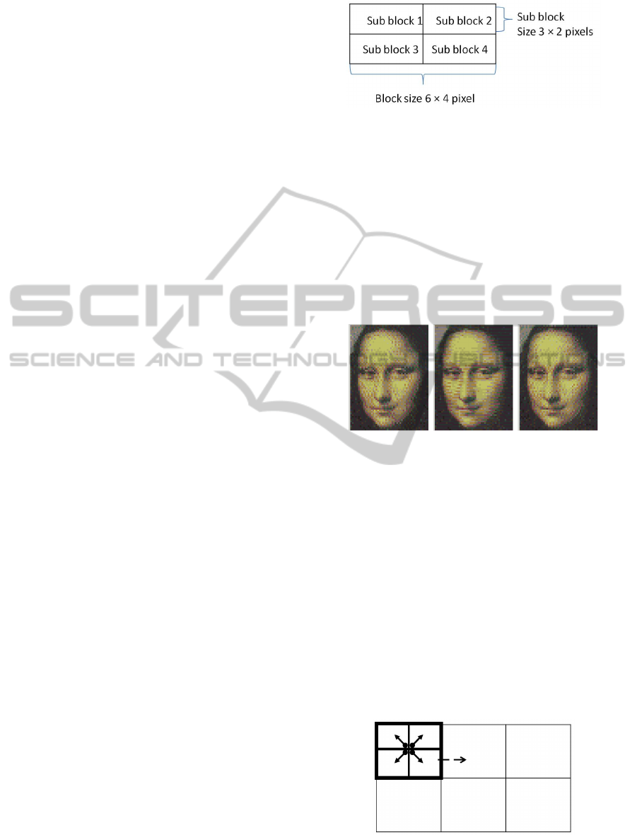
3.1 Block Size
The size of the block is crucial for achieving a good
image quality. Based on our experiments, FWB-FSD
produces the best image quality when k = 1. That is,
the size of each sub-block is 3 × 2 pixels. Unless
otherwise stated, we assume that the default block
size is 6 × 4 pixels.
In the next section we will use other block sizes to
show that the best block size is 6 × 4 pixels for FWB-
FSD. In this section, we will use the sub block size 6
× 4 pixels to explain FWB-FSD.
3.2 Sub-block Parsing Directions
To prevent the latticed and directional appearance in
the output image and keep the structure of the input
image, we observed that the parsing order is critical .
We have explored a number of different parsing
orders and discovered that under a given parsing
Figure 5: An input image divided into blocks, where each
block consists of 4 sub-blocks of equal size, except the
bottom and the right-hand edges.
order, color bandings of different input images would
tend to appear in the same direction. For example,
Figure 6 (a) and (c) are output images obtained from
two different vertical parsing directions: top-down in
(a) and bottom-up in (c). These two output images
both depict vertical directional artifact color bandings.
Figure 5 (b) is an output image obtained from a
horizontal parsing of right to left. It depicts a
horizontal directional artifact color banding.
(a) (b) (c)
Figure 6: Observable directional artifacts: (a) and (c) are
output images from vertical parsing, while (b) is an output
image from a horizontal parsing.
In the FWB error-diffusion scheme each sub-
block in a block is parsed in a different direction.
Sub-block 1 in Figure 5 is parsed bottom-up and from
right to left using FWB-FSD. Sub-block 2 is parsed
top-down and from left to right. Sub-block 3 is parsed
top-down and from right to left. Sub-block 4 is parsed
top-down and from left to right. The directions
between sub-blocks have the effect of asteroid
emission, which prevents double compensation on
one pixel and keeps 4 pixels in each block from being
diffused by other pixels (see Figure 7). This helps to
remain the structure of the input image.
Figure 7: For each block being scanned, FWB parses each
sub-block in a different direction.
IMAGAPP 2011 - International Conference on Imaging Theory and Applications
128
3.3 The Euclidean Distance for
Selecting the Best Color for a Pixel
We want to select the closest color from the given
color palette to that of the original input pixel. Early
research has indicates that perceived differences
between colors are well represented by the Euclidean
distance of the RGB vectors. The color models can
be presented by RGB, MYK, CIEXYZ, CIELAB,
HSB and YIQ.
The application is based on the Microsoft window.
RGB is a device dependent color space of Microsoft
window. HSB is that it often used by artists because
it is often more natural to think about a color in terms
of hue and saturation than in terms of additive or
subtractive color components. HSB is a
transformation of an RGB color space, and its
components and colorimetric are relative to the RGB
color space from which it was derived.
We use the RGB color space and the HSB values
to represent colors. A particular RGB color space is
defined by the three chromaticties of red, green, and
blue. HSB stands for Hue, Saturation, and Brightness,
which is one of the most common cylindrical-
coordinate representations of points in an RGB color
model. HSB rearranges the geometry of RGB that is
more perceptually relevant than the Cartesian
representation. We calculate the closest color using
both RGB and HSB values: We first calculate the
Euclidean distance of RGB value for each pair of a
given input color and a color in the given set of
limited color palette. Select the color with the
smallest distance. If there are two or more such pairs
with the same Euclidean distance, we will compute
the Euclidean distance on the HSB values on these
pairs, and select the one with the smallest distance
In particular, we use c to represent the value in
RGB space. Let c = (
,
,
) be the RGB vector of
a pixel in the input image and X = {(
,
,
) |
=0,…,−1} be the given set of colors in the
color palette.
We want to find the shortest Euclidean distance d.
| =
(
–
)
(
−
)
(
–
)
(2)
where (
,
,
) is one of the colors in X,
=0, …, −1.
If there are two or more colors in X with the same
shortest distance to c, we will calculate the shortest
Euclidean distance of the HSB values of these colors
to the HSB value of c and select the color with the
shortest Euclidean distance of HSB values. Since the
Hue value is much larger, we will first normalize it
(dividing it by 360) to a value between 0 and 1 before
calculating the Euclidean distance.
We may also use rectilinear distance to find the
“closest” color. Shown in Figure 8 are two output
images, where Figure 8 (a) is obtained by finding the
first shortest rectilinear distance difference of the
RGB vectors of c and the colors in X. Figure 8 (b) is
created by finding the shortest Euclidean distances of
both the RGB space and HSB values, which incur
lesser color bandings and result in a smoother image
than Figure 8 (a).
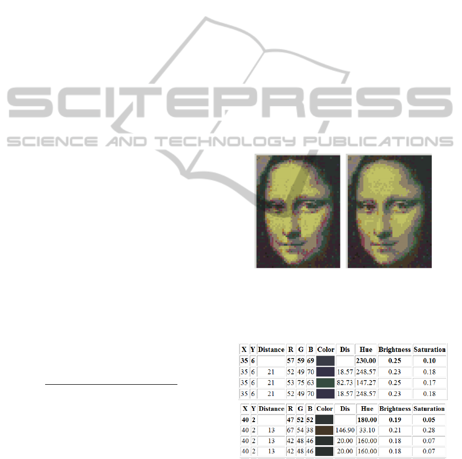
Figure 9 shows two examples of color selection
mechanism used in FWB-FSD. The first row
indicates an input color of RGB space and HSB in the
coordinates x and y. In each of these two examples
there are two colors in the second and third rows with
the same shortest Euclidean distance of the RGB
vector in the original image. The second row in
Figure 9 is selected by the RGB space and has the
same Euclidean distance with the third row. The third
row in Figure 9 is selected by the HSB and has the
same Euclidean distance with second row. With the
help of HSB values, we are able to select the color
that is closest to the original.
(a) (b)
Figure 8: (a) Selecting colors by the shortest rectilinear
distances difference of RGB vectors. (b) Selecting colors by
the shortest Euclidean distances of RGB vectors and HSB
values.
Figure 9: The column Dist is for distance of HSB, H for
Hue, S for Saturation and B for Brightness. The color in the
second row was selected without the HSB values
comparison, while the color in the last row was selected in
Fig. 8 (b), which is closer to the original color.
PRODUCING AUTOMATED MOSAIC ART IMAGES OF HIGH QUALITY WITH RESTRICTED AND LIMITED
COLOR PALETTES
129
3.4 Error Diffusion in Blocks
and Sub-blocks
FWB-FSD uses the FSD error-diffusion coefficient to
parse pixels in each sub-block and distributes the
quantization error to its neighboring pixels. After
selecting the closest color, it diffuses the quantization
error to its neighbors. How neighboring pixels will be
compensated is determined by the locations of the
parsing pixel of sub-block in the block (see Figure
10).
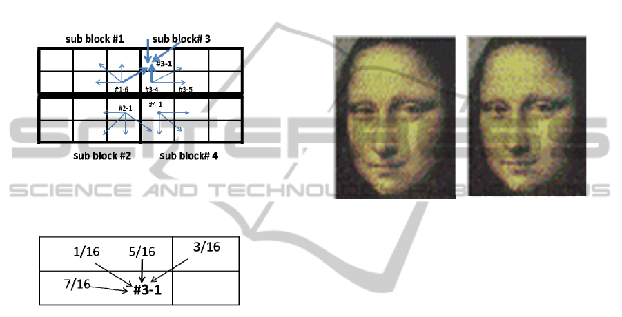
Figure 10: Under FWB-FSD the pixel number 3-1 grains
the different portion of quantization error from different
directions.
Figure 11: The pixel number 3-1 in FSD gets error diffusion
from different quantization error of different pixels in only
one direction.
The portions of quantization error are obtained
differently between pixels depending on the locations
of sub-blocks. We note that if a block is already
parsed, then it will not be parsed by the unprocessed
blocks again. For example, pixel #3-1 shown in
Figure 10 receives 4 portions of error quantization
including the two portions from the sub-block above,
a portion from pixel #1-6, and a portion from pixel
#3-4. Thus, the sequence of the portions it receives
will be 5/16, 3/16, 3/16, and 3/16. Major differences
between FWB-FSD and FSD are that pixel #3-1 in
FWB-FSD receives error diffusions from more
directions than FSD and the pixels #1-6, #3-4, #2-1
and #4-1 shown in Figure 10 keep the same RGB
values without being compensated from other pixels.
There are four cells in the sub block will not
propagate its error-diffusion to its next neighbors.
They are the last cell in the sub block 1 of the first
block, the last cell in the sub block 2 of the last block
of first row, the last cell in the sub block 3 of last row
of the first block and the last cell in the sub block 4 of
the last row of the last block in the image which
comparison with FSD that its last cell in the image.
As the result, FWB-FSD not only better maintain the
image quality without losing too much information of
the input image but also reduce directional and
latticed appearance in the output image. Figure 12
depicts the differences in the output images using
these two methods. The difference is particularly
noticeable in Mona Lisa’s right eye: It is blurry in
Figure 12 (a) under FSD, which looks like half closed.
It is much clearer in Figure 12 (b) under FWB-FSD.
We will provide more details in the next section.
(a) (b)
Figure 12: (a) Output image by FSD. It is clearly noticeable
that Mona Lisa’s right eye is blurry and looks half closed.
(b) Output image by FWB-FSD. The eye problem in (a) is
corrected.
3.5 Running Time
We note that FWB-FSD scans each pixel only once as
in FSD. For each pixel it scans, FWD-FSD carries the
same number of operations as FSD except that FWD-
FSD may be in a different direction. Thus, the
running time of FWD-FSD is the same as FSD.
Likewise, it is easy to see that the running time of
FWD-XYZ is the same as error-diffusion algorithm
XYZ.
4 RESULT AND EVALUATION
Parsing direction plays a crucial role in error-
diffusion dithering for achieving good quality and
retaining detailed information of the input image.
The direction to obtain good quality depends on the
colors of the input image. Thus, using different
directions to diffuse errors can enhance quality of the
output image.
This section presents comparisons of more output
images under FSD and FWB-FSD (see Figures. 13 to
15). We first use images of continuous tone and
different shapes to compare the output images
IMAGAPP 2011 - International Conference on Imaging Theory and Applications
130
produced FWB-FSD and FSD. For images of
extremely simple shape (e.g. a rectangle) of one
continuous simple color, we observe uneven
structure in the output image produced by FWB-FSD
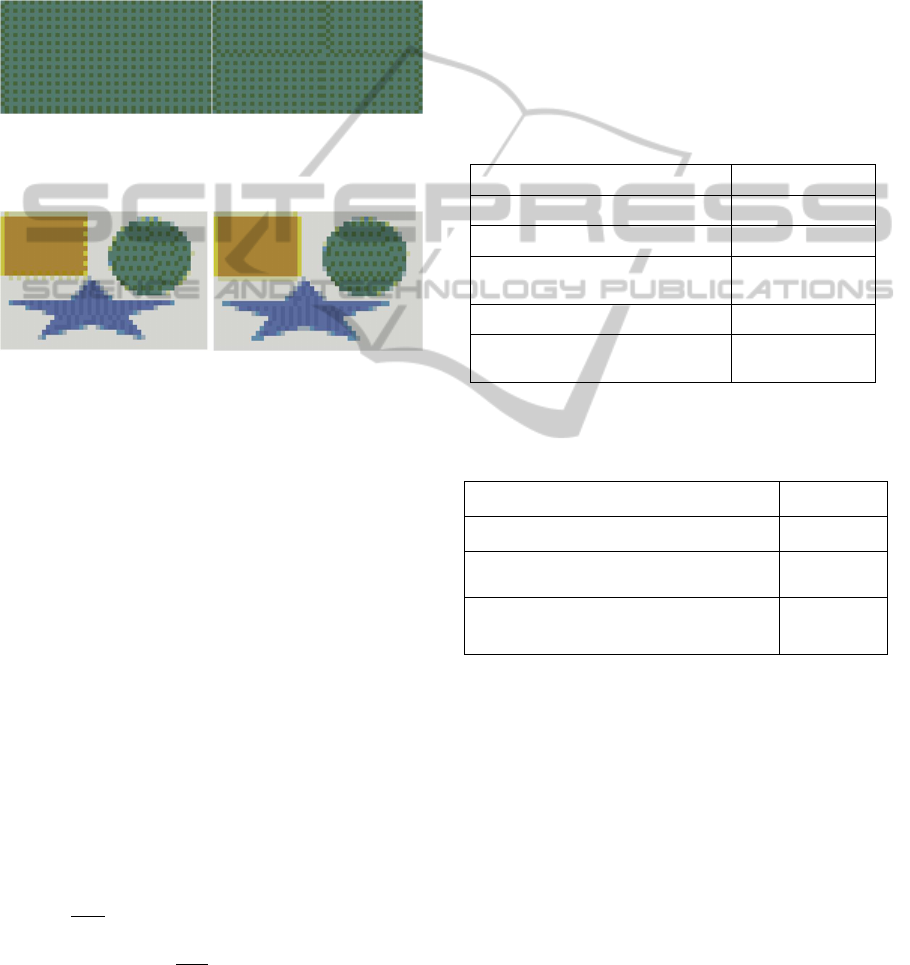
(see Figure. 13). However, for images of simple
shapes (such as rectangles, stars, and circles) with
more colors, FWB-FSD produces much smoother
images than FSD (see Figure 14). The orange square
in the Figure 14 is smoother than left side image.
Figure 13: The left-side image is processed by FSD and the
right-side image is processed by FWB-FSD with one
block.
Figure 14: The left-side image is processed by FSD; the
square of orange color shows an uneven structure. The
right-side image is processed by FWB-FSD with one
block; the square appears smoother.
We also used the peak signal-to-noise ratio
(PSNR) to evaluate the final images processed with
different block sizes. In particular, we will PSNR
values to analyze the quality of the proposed method
and evaluate the optical mixture correctness of the
dithering process (Cheuk-Hong, Oscar, Ngai-Man,
Chun-Hung and Ka-Yue, 2009).
When comparing input images, PSNR is often
used as an approximation to human perception of
reconstruction quality. The PSNR computes the ratio
between two images. This ratio is often used as a
quality measurement between the original and a
reconstruction image. The higher PSNR has the
better quality of the reconstructed image. Denote by
Y(i, j) the input image. The input image produced by
FSD or FWB-FSD is denoted by X(i, j). Denote by w
the width of an image and h its height. The
expression of PSNR is shown below:
=
×
×
∑∑
[|
(
,
)
− (,)|]
=10× log
Table 1 lists the results of PSNRs on the input
image of Mona Lisa (50 × 67 pixels) and its output
images produced by, respectively, FSD and FWB-
FSD with a few reasonable block sizes. Table 2 lists
the results of PSNRs on the original image of Mona
Lisa (136 × 182 pixel) as the input image and its
output images produced by, respectively, FSD, FWB-
FSD with one block and FWB-FSD with block size of
6 × 4 pixels, where FWB-FSD with one block means
to divide the image into four parts of equal size by
connecting the middle points on each side of the
image. We note that FWB-FSD with block size of 6 ×
4 pixels produces the best PSNR. Additional
comparisons are presented in the appendix.
Table 1: The results of PSNRs on the input image of Mona
Lisa (50 × 67 pixels) and its output images.
The algorithm to process value
FSD 22.42
FWB-FSD with one bloc
k
22.53
FWB-FSD with block size 6×4
pixels
22.64
FWB-FSD with block size 12×8pixel 22.46
FWB-FSD with block size
24×16pixel
22.46
Table 2: The results of PSNRs on the original image of
Mona Lisa (136 × 182 pixel) as the input image and its
output images.
The Al
g
orithm to Process Value
FSD 22.54
FWB-FSD with one block 22.68
FWB-FSD with block size 6 × 4
pixels
23.04
5 CONCLUSIONS
The output image generated by FSD tends to be rigid
with directional and latticed appearance, which could
lose the vividness of the original image. This is
undesirable in an art product. The images generated
by FWB-FSD have corrected these problems. We
have demonstrated that our FWB error-diffusion
scheme is a promising new method for achieving
mosaic images of higher quality. We have tested a
large number of other input images not presented
here, and found that FWB-FSD with block size of 6
× 4 pixels always produces the best PSNR values
compared to FSD and FWB-FSD with other block
PRODUCING AUTOMATED MOSAIC ART IMAGES OF HIGH QUALITY WITH RESTRICTED AND LIMITED
COLOR PALETTES
131
sizes.
We note that for PSNR values below 3.00, it is
often difficult for human eyes to detect differences
between two images. But mosaic art images enlarge
each pixel, and so it is easier to observe differences
between two pictures with PSNR value below 3.00.
We have shown that FWB-FSD is a better algorithm
on mosaic art images and other types of images that
require enlargement of pixels. In particular, we found
that the FWB scheme works better when the input
image has abundant colors and is rich in shapes.
Finally, we note that we can use other error-
diffusion algorithms to go with the FWB scheme. For
certain type of images, using a different underlying
error-diffusion algorithm may be more appropriate
than using FSD.
ACKNOWLEDGEMENTS
This work was supported in part by the NSF under
grant CCF-0830314.
REFERENCES
Bayer, B., 1976, Color imaging array. U.S. patent
3,971,065 .
R. Floyd and L. Steinberg, 1975. An adaptive algorithm for
spatial grey scale, SID Intl. Svmp. Dig. Tech. Papers
VI, 36—37.
F. Jarvis, C. N. Judice and W. H. Ninke, 1976 , A Survey of
Techniques for the Display of Continuous Tone
Pictures on Bi-level Displays. Computer Graphics and
Image Processing, 5 13–40.
Jeng-Nan Shiau and Zhigang Fan, 1993, Method
forQuantization Gray level Pixel data with extended
distribution set, United States Patent, Patent number
5,353,127.
P. Stucki, MECCA, 1981, a multiple error correcting
computation algorithm for bi-level image hard copy
reproduction. Research report RZ1060, IBM Research
Laboratory, Zurich, Switzerland.
Daniel Burkes, 1988, Presentation of the Burkes error
filter for use in preparing continuous-tone images for
presentation on bi-level devices, in LIB 15
(Publications), CIS Graphics Support Forum.
Bill Atkinson, 2003, private correspondence with John
Balestrieri, January
T. Riemersma, 1998, A Balanced Dither Algorithm, C/C++
Users Journal, volume 16, issue 12.
Victor Ostromoukhov, 2001, A Simple and Efficient
Error-Diffusion Algorithm. In Proceedings of
SIGGRAPH 2001, in ACM Computer Graphics,
Annual Conference Series, pp. 567-572.
N. Damera-Venkata, B.L. Evans, 2001, FM halftoning via
block error diffusion, proceedings of the 2001
International Conference on Image Processing,
Caca Labs., 2010 http://caca.zoy.org/.
Sam Hocevar and Gary Niger, 2008. Reinstating Floyd-
Steinberg: Improved Metrics for Quality Assessment of
Error Diffusion Algorithms, ICISP 2008, LNCS 5099,
PP. 38-45.
Cheuk-Hong Cheng, Oscar C. AU, Ngai-Man Cheung,
Chun-Hung Liu, Ka-Yue YIP, 2009, Low Color Bit-
depath Image Enhancement by Contour-Region Dither,
Communications, Computers and Signal Processing,
2009 , Page(s): 666 – 670. 2009
APPENDIX
D
EMONSTRATION OF
M
OSAIC
A
RT
I
MAGES
We present four examples of mosaic art images using
FWB-FSD and compare them with the images
generated by FSD (see Figure 15, 16, 17). The
images shown in Figure 17 and 18 are the simulated
mosaic art images while Figure 18 is the real mosaic
art made by a total of 3,350 pieces of 1cm × 1cm
tiles.
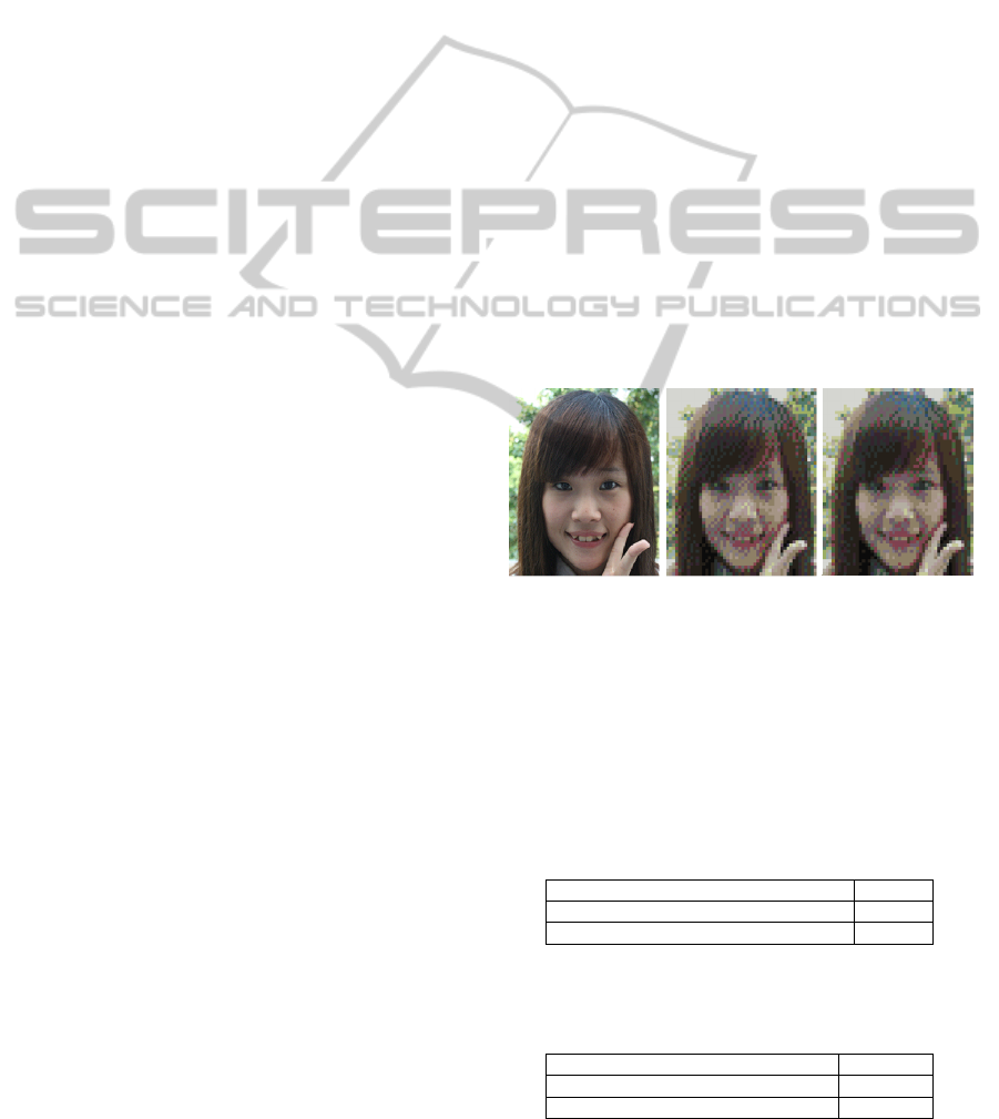
(a) (b) (c)
Figure 15: (a) The input image. (b) The output image with
size 50 × 59 pixels generated by FSD. (c) The output
image of the same size generated by FWB-FSD. Image (b)
has the error quantization diffused to neighbor pixels that
destroy the structure of the mouth. It has the latticed and
unstructured look surrounding the mouth and cheeks.
Image (c) is much better than Image (b) in all aspects.
Table 3: The results of PSNRs on the input image shown in
Figure 16(b) and 16(c), both comparing the output image
with the original image.
The algorithm to process Value
FSD 24.14
FWB-FSD with block size 6×4 pixels 24.48
Table 4: The results of PSNRs on the input image shown in
Figure 17(b) and 17(c), both comparing the output image
with the original image.
The algorithm to process value
FSD 24.13
FWB-FSD with block size 6×4 pixels 24.85
IMAGAPP 2011 - International Conference on Imaging Theory and Applications
132
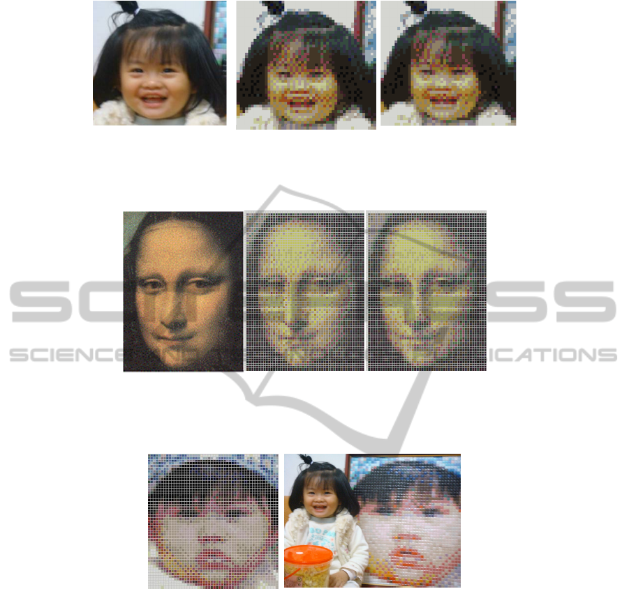
(a) (b) (c)
Figure 16: (a) The input image. (b) The output image with size 50 × 47 pixels generated by FSD. (c) The output image of
the same size generated by FWB-FSD. Image (b) has unstructured cheeks that divide the face into two parts. Image (c) has
corrected this problem.
(a) (b) (c)
Figure 17: Mona Lisa images. (a) Input Image. (b) The output image which simulated mosaic art with 50 × 67 tiles
generated by FSD. (c) The output image which simulated mosaic art with 50 × 67 tiles generated by FWB-FSD. Image (c)
is clearly much better than Image (b).
(a) (b)
Figure 18: (a) The image which simulated mosaic art generated by FWB-FSD. (b) Mosaic Art with size 50 × 67 on 1 cm ×
1 cm square tiles.
PRODUCING AUTOMATED MOSAIC ART IMAGES OF HIGH QUALITY WITH RESTRICTED AND LIMITED
COLOR PALETTES
133
